
Sections
Key message

Background
Physical disturbance can damage seafloor habitats, especially those supporting larger and more fragile species and/or those with longer recovery time. The status of seafloor habitats can be assessed using monitoring data from surveys, ideally across a long time period. However, it is not feasible to monitor the whole seafloor: currently, monitoring data are mostly available from Marine Protected Areas. A modelled approach is necessary for large scale habitat assessments across all Scottish waters. Exposure to pressures associated with human activity can be used to devise a proxy for habitat condition.
This assessment, developed for use in OSPAR and UK Marine Strategy assessments (known as ‘Extent of Physical Damage’ indicator (OSPAR, 2017), predicts the spatial extent and level of physical disturbance by mapping areas where pressures overlap with sensitive habitats. Currently, it only considers disturbance from surface and sub-surface abrasion caused by vessels over 12 m in length using Vessel Monitoring System (VMS) (reporting vessels) fishing with bottom contacting gears. This is considered to be the most significant pressure (Foden, 2011). The corresponding pressure maps produced using these data aggregate pressure across a large grid cell. It is assumed that fishing occurs evenly across the whole grid cell which may not be the case.
The indicator categorises disturbance at the seabed from 0 (none) to 9 (very high). Categories 5 to 9 represent higher levels of disturbance. Areas with a score of 5 and above are considered highly disturbed and, therefore, potentially in poor condition. Habitats may have a high disturbance score if they are heavily fished or, if they are fished less frequently but are highly particularly sensitive to the associated pressures.
This indicator primarily relates to subtidal sediment habitats as rocky areas tend to be avoided by those involved in towed, bottom-contact fishing; however, there will be some disturbance of subtidal rock and reef habitat. Case studies on benthic habitats are available for Loch Creran and Loch Carron and Deep sea vulnerable marine ecosystems.
This assessment covering 2012-2016 supersedes the most recent assessment undertaken for the UK Marine Strategy Assessment, which was at a UK scale and covered 2010 to 2015 (Vina-Herbon et al., 2018). Fisheries data were not available to produce an assessment that covers more recent years.
Data on pressures resulting from human activities and information on sensitivity of habitats are the main components of this indicator. The duration and intensity of the activity, and the physical interaction between the activity and the seabed, are used to define the nature of the pressure assessed in this indicator (Korpinen et al., 2012) (e.g. shipping traffic in deep water does not cause physical disturbance at the seabed).
This method is particularly useful for assessing large sea areas where currently only limited data are available. The European Nature Information System (EUNIS) level 3 classification (Davies et al., 2004) has been used as a proxy for the broad habitats.
Data on pressures alone are not sufficient to assess the likely degree of impact from the physical disturbance. Data on the sensitivity of the habitats to those pressures need to be evaluated in order to determine whether an impact could be occurring. For this assessment, ‘disturbance’ is taken to mean the effect of the different combinations of the pressure varying in intensity and duration on features with variations in natural sensitivities. The specific combination of pressure and sensitivity is used to establish the overall impact (damage) on the habitat.
To distinguish between the different types of pressures caused by fishing gears on seafloor habitats, the penetration depth of different fishing gear components was assessed and classified as either surface or sub-surface abrasion (JNCC, 2011; Church et al., 2016). Surface abrasion pressure damages species and communities on the surface and upper layers of sediment, for example calcareous algae growing on the surface of gravels. Sub-surface abrasion pressure is defined as the penetration of the substrate to more than 3 cm below the surface, damaging species and communities living within the sediment such as burrowing bivalves. The gear types included in this assessment, and which can be assigned surface and sub-surface pressures are:
- Beam trawl
- Nephrops trawl
- Otter trawl
- Dredge (including scallop dredge)
- Demersal seine
The current results are based on surface and sub-surface abrasion from reporting vessels during the 2012–2016 assessment period only. It should be noted that Vessel Monitoring System (VMS) data from vessels 12–15 m long became progressively more available through this five-year period. All available data were included, but the assessment will underestimate pressure for vessels within this size range.
Impacts from smaller vessels and information on other human activities causing physical damage to the seafloor will be considered for inclusion in future assessments as the methodology develops.
The extent of physical damage indicator uses two types of information:
- the distribution and sensitivity of habitats (resilience and resistance), and
- the distribution and intensity of human activities and pressures that cause physical damage, such as mobile bottom gear fisheries, sediment extraction and, construction/developments, although only fisheries is covered in this assessment.
These two sources of information (pressure and sensitivity) are combined to predict the disturbance to a given seafloor habitat across the five-year period. The current assessment considered the 2012 to 2016 period, therefore, data on disturbance that took place before this period were not included.
The components of the analysis are:
- A composite habitat map showing the extent and distribution of seabed habitats (based on observational and modelled data), including the mapped extent of any relevant features such as records and distribution of particular species and biotopes like EUNIS level 5 habitats or other biological characteristics. For this assessment, a biotope is defined as ‘the combination of an abiotic habitat and its associated community of species’ (Connor et.al, 2004). All habitat data were combined at EUNIS level 3.
- Tables relating benthic habitat types to habitat sensitivity scores based on their resistance and resilience (recoverability) (Tillin et.al, 2010; Tillin et.al, 2010; BioConsult, 2013; Tillin & Tyler-Walters, 2014). The sensitivity is assessed at species, biotope and EUNIS level 3 level (broad-scale habitat classification), depending on what habitat mapping information is available.
- Distribution and intensity of pressures causing physical damage. This analysis focussed on surface and subsurface abrasion caused by towed, bottom-contact fishing (for fishing from vessels greater than 12m only) within 0.05° grid cells. Grid cell size is given in degrees due to the curvature of the earth and allowing comparison between geographical areas. Due to variances in latitude, the extent of the 0.05º grid cell differs in total size across the assessment area. The method assumes an even spread of fishing pressure within the grid cell. More spatially accurate data cannot be used due to the sensitivity of the information (Johnson, 2011; ICES, 2015; Church et.al, 2016).
- Distribution of levels of disturbance per habitat type within years. Calculation of disturbance based on the three previous elements: intensity and duration of pressures, and habitat sensitivity per pressure type. Note that the pressures of abrasion (non-fisheries, as well as fishing by reporting vessels), siltation and selective extraction, are not currently included in the assessment, but will be incorporated in future developments of the indicator.
The indicator method is based on a series of four analytical steps to combine the distribution and intensity of physical pressures (component 3) with the distribution and range of habitats (component 1) and their sensitivities (component 2). Data generated by the first three components above are combined using a step-wise approach to calculate the fourth component, which enables the total area of different levels of predicted disturbance and a combination of those, across the sub-region, per habitat type to be estimated. The results are also used to calculate the levels of variability of fishing intensity and identify trends in disturbance per year across a five-year period.
The spatial assessment of this indicator is summarised per EUNIS level 3 polygon and has been prepared by combining the sensitivity and exposure to pressure data for habitats, biotopes, and species within the EUNIS level 3 habitat polygons.
Step 1: Extent of habitats
An important component of this indicator is the production of a composite habitat map showing the extent and distribution of habitats and their associated sensitivities. This map is produced using a combination of benthic survey data and modelled habitat maps. As a basis for the assessment, a full coverage EUNIS level 3 habitat map has been produced for the Scottish inshore and offshore regions, integrating maps from surveys and broad-scale models (Figure a).

The EUNIS habitats are mapped at different levels of detail depending on the information available, from level 3 physical habitats to level 6 biological communities and then aggregated to EUNIS level 3. The majority of the habitat maps were obtained from the European Marine Observation and Data Network Seabed Habitats portal, including the broad-scale physical habitat map known as EUSeaMap (EMODnet, 2010, Seabed Habitats Map Viewer) and more detailed habitat maps created from survey data available. The specification for a habitat map for the assessment of this indicator included the following conditions, to:
- contain information on the relevant EUNIS habitat/biotope type at any level between levels 3 and 6.
- refer data on biotopes to level 3 of the EUNIS habitat classification system.
- use the broad-scale modelled map, EUSeaMap at EUNIS level 3 when higher resolution maps from surveys are not available.
- use the best available evidence on habitat data.
- contain no overlaps.
Mapping rules were established to decide objectively which of the overlapping datasets would be the sole occupant in the overlapping area. Where a EUNIS habitat map developed from survey data overlapped with the EMODnet broad-scale habitat map, a threshold confidence score of 58% was used as a simple rule for deciding whether or not to favour the habitat map from the survey. This threshold was based on the Mapping European Seabed Habitats protocol (EMODnet, 2010).
Within the Mapping European Seabed Habitats scoring system, for any map to have a score greater than 58%, the survey techniques must have used a combination of remote sensing and ground-truthing to derive the habitat types, hence physical and biological elements are included for its production. Therefore, 58% was deemed to be the lower threshold at which an overlapping survey map is considered to be of higher quality than the broad-scale predictive map. Pre-processing conditions and rules for the combining of data are available in the OSPAR Co-ordinated Environmental Monitoring Programme guidelines (OSPAR, 2017).
Step 2: The assessment of habitat sensitivity
The sensitivity of benthic habitats is determined based on a combination of the resistance (tolerance) and resilience (recoverability) of key structural, functional and characterising species of the habitat in relation to a defined intensity of each pressure (Tillin et.al., 2010; BioConsult, 2013; Tillin & Tyler Walters, 2014). Due to data limitations, the sensitivity scores are defined using a categorical scoring approach (Tillin et.al., 2010). Sensitivity assessments for ecological groups have also been undertaken using Bray-Curtis cluster similarity analysis and Multi-Dimensional Scaling, where resistance and resilience scores are assigned to groups of species with similar biological traits, such as burrowers (Tillin & Tyler-Walters, 2014).
The sensitivity map is created with three stages, using best available evidence where present:
- Species records from survey data, that match a list of species assigned to a specific ecological group, are mapped using their maximum sensitivity value (based on the combination of resilience and resistance) for the specific pressure/activity in question. Data are applied to the intersection between the habitat polygon and a 0.05° grid. Maximum values are selected as a precaution to capture the most sensitive species when the values are aggregated together.
- If there is a high enough density of species recorded per habitat area (1 point per 20 km2) and agreement between the species and the underlying habitat they are within, the sensitivity from the same species records used in the stage above are used to assign a modal sensitivity to the surrounding habitat polygon. For example, if data coverage is sufficient, and the substrate and habitat type in the surrounding polygons are the same, then the same sensitivities are applied to these areas.
- Finally, to act as a background map, and to fill in areas not covered by the first two steps, the EUNIS level 3 habitat map is used to assign habitat sensitivities to the whole area. The sensitivities used in this step often cover a range of values (from very low sensitivity to very high), in which case the maximum sensitivity is selected.
The maps are then combined geographically to show the highest confidence information across all regions (Figures b and c in Results: Read More). For a more detailed explanation of the method, please refer to the Co-ordinated Environmental Monitoring Programme guidelines (OSPAR, 2017).
Step 3: The assessment of the extent and distribution of physical damage pressures
Towed, bottom-contact fishing activity is known to be affecting a large area of the seafloor (Dinmore et al., 2003; Eastwood et al., 2007; Foden et al., 2010; 2011; Johnson, 2011; Jennings et al., 2012) so the assessment method currently focuses on the corresponding pressures, surface abrasion (disturbance to seafloor surface features) (Figure d in Results: Read More) and subsurface abrasion (penetration and/or disturbance of the substrate below the surface of the seafloor) (Figure e in Results: Read More). At present other activities, which could cause physical damage pressures, are not included.
Pre-processed aggregated Vessel Monitoring System fishing data are used to calculate the ‘swept area’ of a specific group of fishing gears. The swept area is calculated using the parts of the fishing gear in contact with the seabed, and it is calculated on the width of fishing gear (in metres) multiplied by the average vessel speed (in knots) and the time fished. This calculation is undertaken on a cell-by-cell (0.05° grids or c-squares) basis per gear and per year, using data covering five years from 2012 to 2016. Only the part of gear in contact with the seafloor is used for the analysis (Eigaard et al., 2015; Church et al., 2016). The swept area ratio (proportion of cell area swept per year) is then calculated by dividing the swept area by the grid cell area.
Fishing effort is classified with an intensity scale ranging from ‘none’ to ‘very high’ (cell area swept more than 300% or 3 times per year). A change of three categories or more on the fishing pressure in the same grid across years is considered to be highly variable. The maximum or 95-percentile was not chosen to avoid overestimating the pressure. For a more detailed explanation of the method, the reader is referred to the Co-ordinated Environmental Monitoring Programme guidelines (OSPAR, 2017).
Step 4: The combination of pressure intensity and habitat sensitivity
The degree of disturbance of a habitat is a prediction based on the predicted spatial and temporal overlap of its sensitivity and exposure to a specific pressure. Sensitivity and pressure are combined via a matrix, producing 10 categories of disturbance (0-9, where 0 is no disturbance, and 9 is the greatest amount of disturbance possible). The matrix was created from the result of previous studies that looked at the impacts of pressures on sensitive species and habitats when applied at different levels of intensities (Schroeder et al., 2008; BioConsult. 2013). The matrix is used to calculate the disturbance per cell for each surface and subsurface abrasion per year.
These disturbance maps are then combined by selecting, for each cell the highest disturbance category from the two disturbance layers. The disturbance from surface and subsurface abrasion produce disturbance that overlaps between pressure types. The maximum is, therefore, chosen to prevent double counting (Figure 1 in Results section). For a more detailed explanation of the method, the reader is referred to the Co-ordinated Environmental Monitoring Programme guidelines (OSPAR, 2017).
Disturbance values across years are combined using the aggregated fishing pressure spatial layers, developed in Step 3 above. Results are used to calculate trends between years in those grid cells or c-squares identified as variable. This allows the variation of disturbance across years per habitat type to be assessed. The trend analyses are simple plots over the 6-year period, rather than a linear regression, which was not possible due to the small number of years assessed.
The disturbance categories were aggregated into two groups:
- disturbance categories 0 to 4, representing low levels of disturbance.
- disturbance categories 5 to 9, representing high levels of disturbance.
This scale is the result of a combination of the variation in fishing activity and the range of sensitivity values. The percentage of areas with vulnerable habitats can be calculated based on an assessment of moderate or greater vulnerability for each sub-regional sea (disturbance categories 5-9), as well as by habitat type. Percentage values were calculated for each Scottish / Offshore Marine Region, to compare against a threshold of 15%, which was set as a potential indicator target in 2012 (HM Government, 2012). For a more detailed explanation of the method, the reader is referred to the Co-ordinated Environmental Monitoring Programme guidelines (OSPAR, 2017).
The traffic light assessment for this report has been adapted from the method that was used to assess whether Good Environmental Status (GES) was met for the UK Marine Strategy (Vina-Herbon et al., 2018). A habitat was considered to meet GES if the area in high disturbance categories was above a threshold of 15 %. Failing to meet GES was considered equivalent to a Red score for this assessment. A Green score was defined as an area having no known disturbance. The scoring system is outlined in Table a.
| Score | Threshold |
| Red | >=15% area of region in high disturbance category (5-9) |
| Amber | <15% area of region in high disturbance category (5-9) |
| Green | No known disturbance |
Results
Figure 1 shows the combined disturbance from both surface and subsurface abrasion caused by towed, bottom-contacting fisheries for Scottish waters. Categories 5 to 9 are considered to represent high levels of disturbance. Disturbance was widespread across most Scottish Marine Regions and Offshore Marine Regions. Table 1 shows the proportion of each region where high disturbance is predicted.
When interpreting these results, it should be noted that the pressure data layers used to derive disturbance aggregate pressure across a large grid cell and it is assumed that fishing occurs across the whole grid cell which may not be the case. The percentages provided should be taken as indicative values for disturbed area as they are calculated from the gridded data. High disturbance categories accounted for 1% (Hatton) to 95% (East Shetland Shelf) of the total area of the region. The whole of the East Shetland Shelf (95% high and 5% low disturbance) and Fladen and Moray Firth (86% high and 14% low disturbance) offshore regions experienced some disturbance.
The threshold used for the Marine Strategy was that less than 15% of the habitat area should be in poor condition (Vina-Herbon et al., 2018). The high disturbance categories of 5 - 9 are taken as a proxy for ‘poor condition’. Based on the results of this Scottish assessment, Hatton, Faroe-Shetland Channel and Bailey regions are below the threshold with less than 15% of the area assessed as highly disturbed, while all other regions are above the threshold.
.")
|
Scottish Marine Region (SMR)
|
No predicted disturbance
|
Low disturbance (categories 1-4)
|
High disturbance (categories 5-9)
|
|
Solway
|
12%
|
66%
|
22%
|
|
Clyde
|
8%
|
26%
|
65%
|
|
Argyll
|
20%
|
36%
|
44%
|
|
West Highlands
|
8%
|
27%
|
65%
|
|
Outer Hebrides
|
36%
|
31%
|
33%
|
|
North Coast
|
5%
|
46%
|
49%
|
|
Orkney Islands
|
10%
|
48%
|
41%
|
|
Shetland Isles
|
4%
|
16%
|
80%
|
|
Moray Firth
|
9%
|
34%
|
57%
|
|
North East
|
5%
|
44%
|
51%
|
|
Forth and Tay
|
13%
|
39%
|
48%
|
|
Offshore Marine Region (OMR)
|
|
|
|
|
Hatton
|
98%
|
0%
|
1%
|
|
Rockall
|
61%
|
3%
|
36%
|
|
Bailey
|
87%
|
1%
|
11%
|
|
Hebrides Shelf
|
23%
|
37%
|
40%
|
|
North Scotland Shelf
|
8%
|
28%
|
64%
|
|
Faroe Shetland Channel
|
89%
|
1%
|
10%
|
|
North & West Shetland Shelf
|
2%
|
8%
|
89%
|
|
East Shetland Shelf
|
0%
|
5%
|
95%
|
|
Fladen and Moray Firth Offshore
|
0%
|
14%
|
86%
|
|
Long Forties
|
4%
|
59%
|
36%
|
There are no comparable results from the last Marine Atlas assessment (Baxter et al., 2011) to make a comparison and assess change over time. It is not possible to compare the results of the indicator with an assessment for the last reporting period as any changes in disturbance would reflect mostly changes in the amount of reported fisheries activity VMS data.
The method for assessing whether Good Environmental Status is met for this indicator for the Marine Strategy (Vina-Herbon et al., 2018) was adapted to produce the traffic light assessment for this report. The threshold of 15 % area in high disturbance categories was reused to distinguish between categories. The scoring system is outlined in Table 2.
EUNIS level 3 broad scale habitat maps were produced to be used in the method to assess disturbance (Figure a in Assessment method section). These provide useful context on the distribution of habitats and how this links to sensitivity to bottom fishing.
For alternative scale EUNIS level 3 benthic habitat mapping click on the images below.
 EUNIS Level 3 Habitat - Legend |
")


Sensitivity maps were produced based on the broad scale habitat map and species records (Figures b & c). The sensitivity score assigned to broad scale habitats is often a range of possible values and, as the highest score is selected for modelled areas of the map to be precautionary, the sensitivity may be overestimated in some places. More accurate sensitivity scores can be assigned where species records from point data are available. Sensitivity is expressed in categories from 1-5, where 1 is the least sensitive and 5 is the most sensitive. All areas mapped as broad scale habitats have a sensitivity score of at least 3 (medium) and deep-sea habitats tend to have a sensitivity score of 5 (very high) as deep-sea species are often slow growing so take longer to recover.


For alternative scale mapping click on the images below.
| Benthic habitat and species sensitivities to surface abrasion |


| Benthic habitat and species sensitivities to sub-surface abrasion |


Pressure maps using data from 2012 to 2016 showed pressure and disturbance caused by bottom fishing activities to be widespread within Scottish waters, occurring to some degree in all regions (Figures d & e). However, bottom fishing is absent in large parts of the Hatton, Faroe Shetland Channel and Bailey regions. Surface abrasion is high or very high in a large proportion of Scottish waters, particularly in East Shetland Shelf (88%), Fladen and Moray Firth Offshore (77%), North and West Shetland Shelf (70%), Shetland Isles (66%) and Clyde (61%). High or very high sub surface abrasion occurs over a smaller area overall but was found across over 50% of the Clyde region and nearly 30% of the West Highlands region.
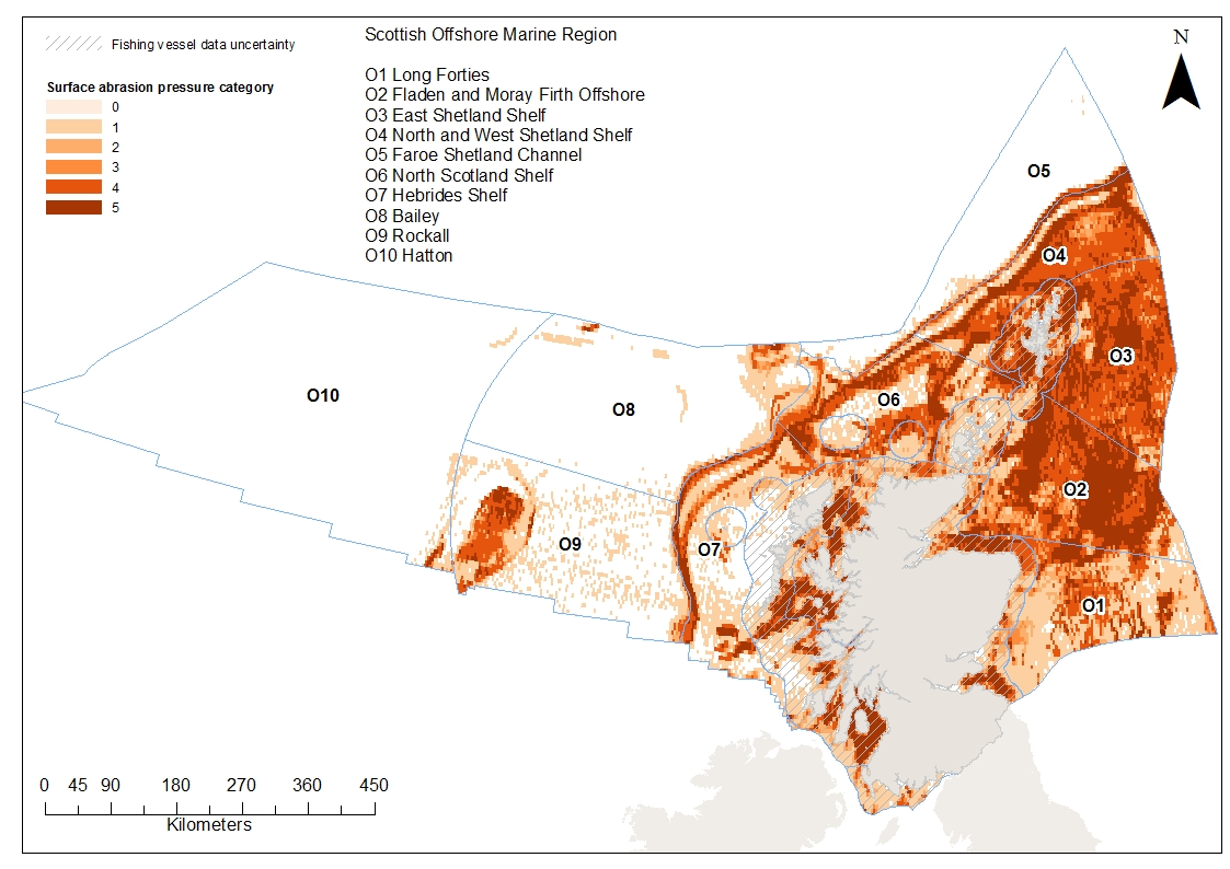
Figure d: Aggregated surface abrasion pressure in regions using 2012-2016 data series. Pressure unit is swept area ratio (the proportion of grid cell swept by fishing gear). Hash indicates inshore areas where fishing data are uncertain due to lack of information for small vessels.
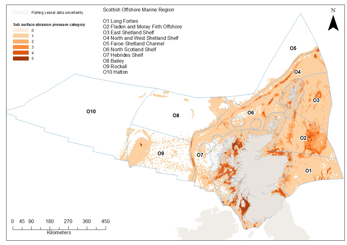
Figure e: Aggregated subsurface abrasion pressure in regions using 2012-2016 data series. Pressure unit is swept area ratio (the proportion of grid cell swept by fishing gear). Hash indicates inshore areas where fishing data are uncertain due to lack of information for small vessels.
For alternative scale mapping click on the images below.
| Aggregated surface abrasion pressure |


| Aggregated sub-surface abrasion pressure |


Figure 1 in the Results section shows the combined disturbance from both surface and subsurface abrasion caused by bottom fisheries for Scottish waters. Finer resolution disturbance maps are available for nearshore regions. The hash indicates inshore areas where fishing data are uncertain due to lack of information for small vessels.
For alternative scale disturbance mapping click on the images below.


Conclusion
Towed, bottom-contacting fishing activities are widespread in most Marine Regions and are capable of causing disturbance to sensitive seabed habitats. Disturbance of seafloor habitats from towed, bottom-contacting fishing activity is predicted to occur to some degree in all regions. The only regions which lack significant disturbance, and which the indicator does not predict to have benthic habitats in poor condition, are in deeper waters off the edge of the continental shelf. Nine out of 21 regions have seafloor habitats which are predicted to be in poor condition across more than half of their area.
Some limitations should be noted when interpreting the results. It is likely that pressure in inshore waters is underestimated due to a lack of fisheries activity data for smaller vessels (data from vessels 12-15 m in length became progressively more available through the assessment period but data for smaller <12 m vessels was not available). Disturbance overall may be overestimated in some places because a precautionary approach was used for assessing sensitivity where data on the distribution of habitats and species were lacking, and the scale of available data on fishing activity means that pressures are assumed to be acting over an area that is likely to be larger than that which is actually fished.
Knowledge gaps
Increased availability and improved resolution of habitat survey data and fisheries data would improve the accuracy of indicator results. Scottish Government have made a commitment (Scottish Government, 2019) for introducing tracking technology for vessels less than 12 m which will result in significant improvements in the inshore waters in future. In situ monitoring data could be used to assess habitat condition over time in a different way, and also assess the accuracy and inform future development of this type of proxy assessment.
The indicator currently only considers disturbance from surface and sub-surface abrasion caused by reporting vessels (those over 12 m in length and using VMS) fishing with bottom contacting gears (considered to be the most significant pressure); however, there is an ambition to add other pressures in the future. Data were not available for some bottom contact fisheries, most notably smaller vessels (<12 m) operating mainly in coastal waters that are not equipped with a Vessel Monitoring System (VMS) transmitter. This means disturbance maps may be an underestimate in some locations. The pressure maps used show aggregated fishing pressure across a large grid cell; is not possible to determine if the same level of disturbance is actually present across the entire cell.
There is low confidence in the habitat data used across a large amount of the assessed area as it is based on models, but medium to high confidence in well surveyed areas such as within Marine Protected Areas. Confidence in the sensitivity scores used depends on the level of data used and the quality of information available on the resistance and resilience of habitats and species to physical damage pressures. Sensitivity scores derived from experimental or field survey studies have high confidence, whereas scores based on expert judgments have low confidence.
Status and trend assessment
|
Region assessed |
Status with confidence |
Trend with confidence |
|---|---|---|
|
All Scotland |
 |
NT |
|
Region assessed |
Status with confidence |
Trend with confidence |
|---|---|---|
|
SMRs |
||
|
Argyll |
|
NT |
|
Clyde |
|
NT |
|
Forth and Tay |
|
NT |
|
Moray Firth |
|
NT |
|
North Coast |
|
NT |
|
North East |
|
NT |
|
Orkney Islands |
|
NT |
|
Outer Hebrides |
|
NT |
|
Shetland Isles |
|
NT |
|
Solway |
|
NT |
|
Western Islands |
|
NT |
|
Region assessed |
Status with confidence |
Trend with confidence |
|---|---|---|
|
OMRs |
||
|
Bailey |
 |
NT |
|
East Shetland Shelf |
|
NT |
|
Faroe-Shetland Channel |
|
NT |
|
Fladen and Moray |
|
NT |
|
Hatton |
|
NT |
|
Hebrides Shelf |
|
NT |
|
Long Forties |
|
NT |
|
North and West Shetland Shelf |
|
NT |
|
North Scotland Shelf |
|
NT |
|
Rockall |
|
NT |
This Legend block contains the key for the status and trend assessment, the confidence assessment and the assessment regions (SMRs and OMRs or other regions used). More information on the various regions used in SMA2020 is available on the Assessment processes and methods page.
Status and trend assessment
|
Status assessment
(for Clean and safe, Healthy and biologically diverse assessments)
|
Trend assessment
(for Clean and safe, Healthy and biologically diverse and Productive assessments)
|
||
|---|---|---|---|
| |
Many concerns |
No / little change |
|
| |
Some concerns |
Increasing |
|
 |
Few or no concerns |
Decreasing |
|
 |
Few or no concerns, but some local concerns |
No trend discernible |
|
 |
Few or no concerns, but many local concerns |
All trends | |
 |
Some concerns, but many local concerns |
||
 |
Lack of evidence / robust assessment criteria |
||
| Lack of regional evidence / robust assessment criteria, but no or few concerns for some local areas | |||
 |
Lack of regional evidence / robust assessment criteria, but some concerns for some local areas | ||
| Lack of regional evidence / robust assessment criteria, but many concerns for some local areas | |||
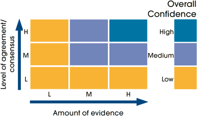
Confidence assessment
|
Symbol |
Confidence rating |
|---|---|
|
Low |
|
|
Medium |
|
|
High |
Assessment regions
 and the Scottish Offshore Marine Regions (OMRs, O1 – O10)")
Key: S1, Forth and Tay; S2, North East; S3, Moray Firth; S4 Orkney Islands, S5, Shetland Isles; S6, North Coast; S7, West Highlands; S8, Outer Hebrides; S9, Argyll; S10, Clyde; S11, Solway; O1, Long Forties, O2, Fladen and Moray Firth Offshore; O3, East Shetland Shelf; O4, North and West Shetland Shelf; O5, Faroe-Shetland Channel; O6, North Scotland Shelf; O7, Hebrides Shelf; O8, Bailey; O9, Rockall; O10, Hatton.
 Regions. These have been used as the assessment areas for hazardous substances.")
, Regions.")