
Background
Species diversity, or biodiversity, is a measure of the variety of species present and is an important property of natural systems. The simplest measure of diversity is richness, or the number of species present. The proportion of these species, or evenness is, however, also important for diversity and proportional abundance can be incorporated into measures of diversity that are also known as diversity indices.
Species diversity is often measured because diverse communities are thought to be more resilient, stable and productive than less diverse ones. As no single index adequately summarises the concept of diversity (Morris, 2014), here a range of indices is used to represent diversity within deep-sea fish (or demersal fish assemblages) through time in the Offshore Marine Regions (OMRs) (Figure 1). These are; species richness, the Simpson index and the Shannon index.

Species diversity within a system may be affected by pressures, such as climate change (both through changes in temperature and ocean acidification); invasive non-native species; pollution and habitat change. Quantifying diversity and assessing changes in it over time is one way that general ecosystem health can be monitored.
This assessment focuses on the diversity of the demersal fish assemblages in the deep-water and offshore areas to the west and north of Scotland. The data used to inform this assessment arose from scientific trawl surveys, the majority of which were conducted from the MRV Scotia. These surveys catch a wide range of fish and all are included in the analysis to measure species richness and the two indices.
Four offshore marine regions (OMR): Bailey, Faroe Shetland Channel (FSC), Hatton and Rockall are considered here (Figure 1). These OMRs occur in two distinct biogeographical areas separated by the Wyville Thompson Ridge (WTR), which lies at around 60 ˚N and acts as a barrier between two water masses. To the north of the WTR, the FSC is exposed to cold Arctic waters, while the remaining OMRs to the south experience warmer Atlantic waters. As a result, the composition of the fish assemblages in these two biogeographical regions are quite distinct.
Rockall Trough, lying to the west of Scotland (making up large parts of the Bailey and Rockall OMRs), is considered the ‘cradle of deep-sea biological oceanography’ due to the pioneering work undertaken here by Victorian scientists in the mid-19th century (Gage, 2001). These early expeditions dispelled the previously held wisdom that these depths were devoid of life. It is now established that fish biodiversity increases between depths of 400 – 1000 m (Clarke et al., 2015).
There is a long history of exploitation of fish stocks in parts of these offshore areas. Rockall Bank, for example, has supported a fishery for more than 200 years (Newton et al., 2008). Deep-water trawl fisheries began operating in the area during the 1970’s, but the rapid increase in commercial exploitation did not begin until 1989 and remained unregulated till 2003 (Gordon, 2003; Clarke et al., 2015).
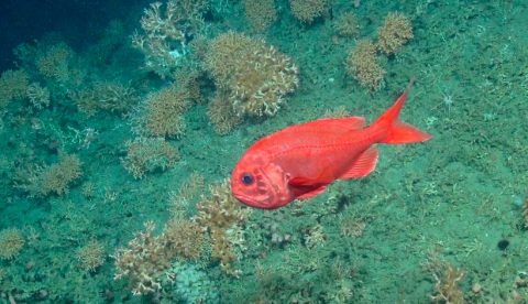
Examples of species that have been commercially exploited in the area include: monkfish (Lophius piscatorius), black scabbardfish (Aphanopus carbo), torsk (Brosme brosme), ling (Molva molva), argentines (Argentina spp.), blue ling (Molva dipterygia), roundnose grenadier (Coryphaenoides rupestris), orange roughy (Hoplostethus atlanticus) and some of the deep-water sharks (mainly leafscale gulper (Centrophorus squamosus) and Portugese dogfish (Centroscymnus coelolepis)) (Campbell et al., 2011, see Priede 2019 for a review of some important deep-water fish species in the area). Several decades of exploitation has resulted in significant declines in the abundance of some of these commercially important species, and even commercial extinction in the case of the orange roughy (Dransfeld et al., 2013).
Management efforts in the area were first introduced through a total-allowable-catch (TAC) management system in 2003 and over subsequent years through gear bans (e.g. gillnets), with the fishery for deep-water sharks phased out in 2010 (Neat et al., 2015). More recently, in an effort to protect vulnerable deep-sea marine ecosystems, the EU introduced a ban on all bottom trawling gears operating below 800 m within its waters (EC, 2016).
The EC’s Marine Strategy Framework Directive (EC, 2008), is the policy framework for the protection of the marine environment and the environmental pillar of the Integrated Maritime Policy. It aims to achieve Good Environmental Status of the EU’s maritime waters by 2020, and to protect the marine resource base upon which economic and social activities depend. It does this by setting out 11 high-level descriptors of environmental status, the first of which aims to: “maintain biodiversity in line with a natural state appropriate for a particular area”. Assessing diversity across time can give an indication of how a system is responding to the pressures placed on it. The diversity of organisms in living systems effects how they respond to changes in the environment, underpins ecosystem function, and provides ecosystem goods and services that benefit humanity, such as the provision of food (Hiddink et al., 2008; Campbell et al., 2011).
The measures of diversity used in this assessment are, briefly:
Species richness
The number of different species present, with no consideration of abundance.
Shannon’s diversity index
This index takes account of both richness and evenness (proportional abundance of each species) and represents the uncertainty surrounding an unknown individual drawn from an assemblage. If an assemblage has high evenness, i.e. where all species are represented by similar numbers of individuals, then identifying an unknown individual has a high associated uncertainty (it may equally be one of a number of species). If, however, the assemblage is uneven, with one or a few species dominating, then the unknown individual may be predicted with less uncertainty as it is more likely to come from one of the dominating species. It is calculated using: -∑Pi ln(Pi), where Pi is the proportion of individuals belonging to species i.
Simpson’s diversity index
This index takes account of both richness and evenness and represents the probability that two randomly chosen individuals belong to different species. It is calculated using: 1 - ∑Pi2, where Pi is the proportion of individuals belonging to species i.
See Magurran (2004) and Morris et al. (2014) for more information.
The data used for this assessment were compiled from various scientific surveys (Table a, Figure a).
|
Data series name
|
From
|
To
|
Offshore Marine Regions
|
Ref / Link
|
|
DATRAS Central Northeast Atlantic Deepwater Trawl Surveys (DWS)
|
1998
|
2018
|
Bailey; Rockall
|
Neat et al., 2010
|
|
Exploratory Seamount
|
2007
|
2007
|
Bailey; Rockall
|
-
|
|
Gear Trials
|
2008
|
2008
|
Bailey; Rockall
|
-
|
|
MOREDEEP 1
|
2014
|
2014
|
Bailey; Faroe Shetland Channel
|
-
|
|
MOREDEEP2
|
2016
|
2016
|
Bailey; Faroe Shetland Channel; Rockall
|
-
|
|
OFFCON Rockall
|
2011
|
2011
|
Rockall
|
-
|
|
OFFCON Rockall 2
|
2012
|
2012
|
Bailey; Hatton; Rockall
|
-
|
|
DATRAS Scottish Bottom Trawl Rockall Survey
|
1998
|
2010
|
Hatton; Rockall
|
|
|
DATRAS Scottish Rockall Groundfish Survey (SCOROC)
|
2011
|
2018
|
Hatton; Rockall
|
|
|
Scottish Irish Anglerfish and Megrim Industry Science Survey (SCO-IVVI-AMISS-Q2)
|
2010
|
2018
|
Bailey; Hatton; Rockall
|
Fernandes et al., 2007
|

Method
During the work undertaken for the 2011 Scottish Marine Atlas (Baxter et al., 2011) no assessment of the wider demersal fish community in the offshore marine regions was made. In an effort to set the results for the current assessment in context, here an assessment for three time periods of seven years each (1998–2004, 2005–2011, 2012–2018) has been made to examine any temporal trends in the wider fish community for the Bailey, Faroe-Shetland Channel, Hatton and Rockall marine regions. Time periods of 7 years were chosen as this is the period of time across which the assessment runs. For the purposes of broad scale assessment, diversity is more meaningfully assessed at a larger spatial scale than the level of individual sampling units. To this end, scientific trawl data were summarised on a regular grid with a cell size chosen by performing a sensitivity analysis as follows:
A grid cell size of 15 km was chosen as optimal based on the sensitivity analysis (Figure b).
 derived through a sensitivity analysis on how the correlation between benthic vertebrate diversity (ICES VME database) and fish diversity changed when varying grid-cell size.")
Results
For the FSC OMR, no data prior to this assessment period (2014–2018) were available. As such, it was not possible to determine any temporal trends. Similarly, the Hatton OMR only had data for the 2005–2011 and current assessment periods and this is restricted to the south-east of the area.
There are no clear trends in species richness across the OMRs (Figure 2). In the Bailey OMR, the 2005–2011 richness value is higher, but also has wide error bars. The elevated values for 2005–2011 at Bailey is likely more an artefact of the patchy sampling than a reflection of any real change in diversity. The FSC OMR has data for the current assessment only. It has notably lower species richness than the other OMRs, but this is expected given the influence of Arctic water in the FSC OMR. For the Hatton OMR, there is a slight increase in species richness for the current assessment period against the 2005–2011 one. However, given there are data for only two time periods and the Hatton OMR has not been sampled extensively, it is not possible to say with any confidence whether this is reflective of a trend. There is no apparent trend for the Rockall OMR and the values across the three time periods are quite stable.
For each OMR a similar pattern to that of species richness is observed for the Simpson (Figure 3) and Shannon (Figure 4) indices, where there are no clear trends across the three time periods. The values for the Simpson and Shannon indices in the FSC OMR are more similar to the other OMRs than for the species richness. This is because evenness (abundance across species) is also factored into these diversity indices. The Rockall OMR has little variation between values through time and appears quite stable, potentially due to the higher levels of survey effort in this OMR. For the Shannon index in particular, however, the Rockall OMR appears to have lower values than the other three OMRs. This is likely a consequence of the relatively shallow nature of the most numerous data on top of Rockall Bank, where the lower diversity at these depths (Figures I, j and k in Read More) has a greater influence on the mean value across the OMR than that of Bailey, for example.
 across the three assessment periods.")
 across the three assessment periods.")
 across the three assessment periods.")
Survey effort has increased during the 3 time periods as observed in the increasing spatial coverage of survey effort throughout the OMRs (apart from Hatton) in more recent periods (Figures c-k). Note that cells with bold colour are where data was available, transparent cells with only the base-map visible are no data cells.
Species richness results are shown in Figures c (1998–2004), d (2005–2011), e (2012–2018).


Simpson Index results are shown in Figures f (1998–2004), g (2005–2011), h (2012–2018).


Shannon’s Index results are shown in Figures i (1998–2004), j (2005–2011), k (2012–2018).


It is clear from the arrangement of data that survey effort has increased through time. Rockall has the least variability between time periods, which is likely due to this OMR being the most surveyed. The survey coverage in the other OMRs is patchier in space and time. This is particularly true for the Hatton OMR, where only the area furthest south-east has been surveyed in any given time period. The results of this assessment should be taken with some caution as it extrapolates over a large area, based on localised sampling and it may take a longer time period for the effects of fishing to become fully apparent (Clarke et al., 2015). Reporting on the Hatton OMR in future assessments will require an increase in survey effort, which will allow a more representative assessment of this region.
Conclusion
There are no clear trends evident in the diversity of the deep-sea fish community across the Bailey and Rockall OMRs as measured by the diversity indices across the time periods assessed here. Our findings are consistent with Campbell et al., 2011, where no temporal trends in community composition were found on the continental slope to the west of Scotland (Bailey and Rockall OMRs).
Knowledge gaps
The offshore marine regions are large areas that have been patchily sampled in space and time, which is a common issue in the deep-sea due to the challenges involved in accessing these areas. In the current assessment, this patchy sampling has necessarily been extrapolated across the entire area of each OMR. The notable gaps in sampling coverage are; the deep regions of the Rockall Trough, the western reaches of the Bailey OMR and the entire Hatton OMR, save the furthest south-east corner. Future sampling in these areas will allow for a more holistic assessment of these OMRs in the future.
Status and trend assessment
|
Region assessed |
Status with confidence |
Trend with confidence |
|---|---|---|
| All regions |
 |
|
|
Bailey |
 |
|
|
Faroe-Shetland Channel |
|
|
|
Hatton |
|
|
|
Rockall |
|
|
This Legend block contains the key for the status and trend assessment, the confidence assessment and the assessment regions (SMRs and OMRs or other regions used). More information on the various regions used in SMA2020 is available on the Assessment processes and methods page.
Status and trend assessment
|
Status assessment
(for Clean and safe, Healthy and biologically diverse assessments)
|
Trend assessment
(for Clean and safe, Healthy and biologically diverse and Productive assessments)
|
||
|---|---|---|---|
 |
Many concerns |
No / little change |
|
| |
Some concerns |
Increasing |
|
 |
Few or no concerns |
Decreasing |
|
 |
Few or no concerns, but some local concerns |
No trend discernible |
|
 |
Few or no concerns, but many local concerns |
All trends | |
 |
Some concerns, but many local concerns |
||
 |
Lack of evidence / robust assessment criteria |
||
| Lack of regional evidence / robust assessment criteria, but no or few concerns for some local areas | |||
 |
Lack of regional evidence / robust assessment criteria, but some concerns for some local areas | ||
| Lack of regional evidence / robust assessment criteria, but many concerns for some local areas | |||
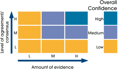
Confidence assessment
|
Symbol |
Confidence rating |
|---|---|
|
Low |
|
|
Medium |
|
|
High |
Assessment regions
 and the Scottish Offshore Marine Regions (OMRs, O1 – O10)")
Key: S1, Forth and Tay; S2, North East; S3, Moray Firth; S4 Orkney Islands, S5, Shetland Isles; S6, North Coast; S7, West Highlands; S8, Outer Hebrides; S9, Argyll; S10, Clyde; S11, Solway; O1, Long Forties, O2, Fladen and Moray Firth Offshore; O3, East Shetland Shelf; O4, North and West Shetland Shelf; O5, Faroe-Shetland Channel; O6, North Scotland Shelf; O7, Hebrides Shelf; O8, Bailey; O9, Rockall; O10, Hatton.
 Regions. These have been used as the assessment areas for hazardous substances.")
, Regions.")