Winter nutrient concentrations

Sections

Key message

There was no statistically significant increase in the winter nutrient concentrations during the period 2007 to 2019 in any of the Scottish Marine Regions (SMRs) and concentrations are at levels that cause no concern.

Winter storm

PDF Summary

Background

Eutrophication in the marine environment is the excessive growth of phytoplankton in response to enrichment by nutrients resulting in an undesirable disturbance in the marine ecosystem. The consequences are often wide ranging, with overall impacts on the diversity and abundance of flora and fauna resulting from the depletion of oxygen in the water column, increases in water turbidity and behavioural changes in larger fauna. However, nutrients such as dissolved inorganic nitrogen (DIN), dissolved inorganic phosphorus (DIP) and dissolved silicate (DSi) also occur naturally and are essential for primary production supporting the marine food web.

The main source of silicate in the marine environment is from the weathering of rocks, therefore local geology will influence silicate concentrations. Anthropogenic sources of nitrogen and phosphorous, including agricultural run-off and domestic and industrial waste discharges can result in elevated nutrient concentrations, particularly in coastal waters. Nutrient concentrations in Scottish waters exhibit a seasonal cycle, typical of northern latitudes. Phytoplankton (microscopic marine algae) biomass increases in the spring due to the increase in light and water column stability, and nutrient concentrations decrease as they are utilised by phytoplankton for growth. Low light intensity and increased turbulence during winter limit phytoplankton growth and nutrients accumulate in the water column. In offshore waters nutrient concentration can also vary systematically with depth, with higher concentrations often found in deeper water below the light zone.

Marine Scotland Science (MSS) collect water samples to determine winter nutrient concentrations on an annual basis. Data produced are used in eutrophication assessments for OSPAR and the EU Marine Strategy Framework and Water Framework Directives.

This assessment evaluates winter nutrient concentrations and trends in the Scottish Marine Regions (SMRs) from 2007 to 2019.

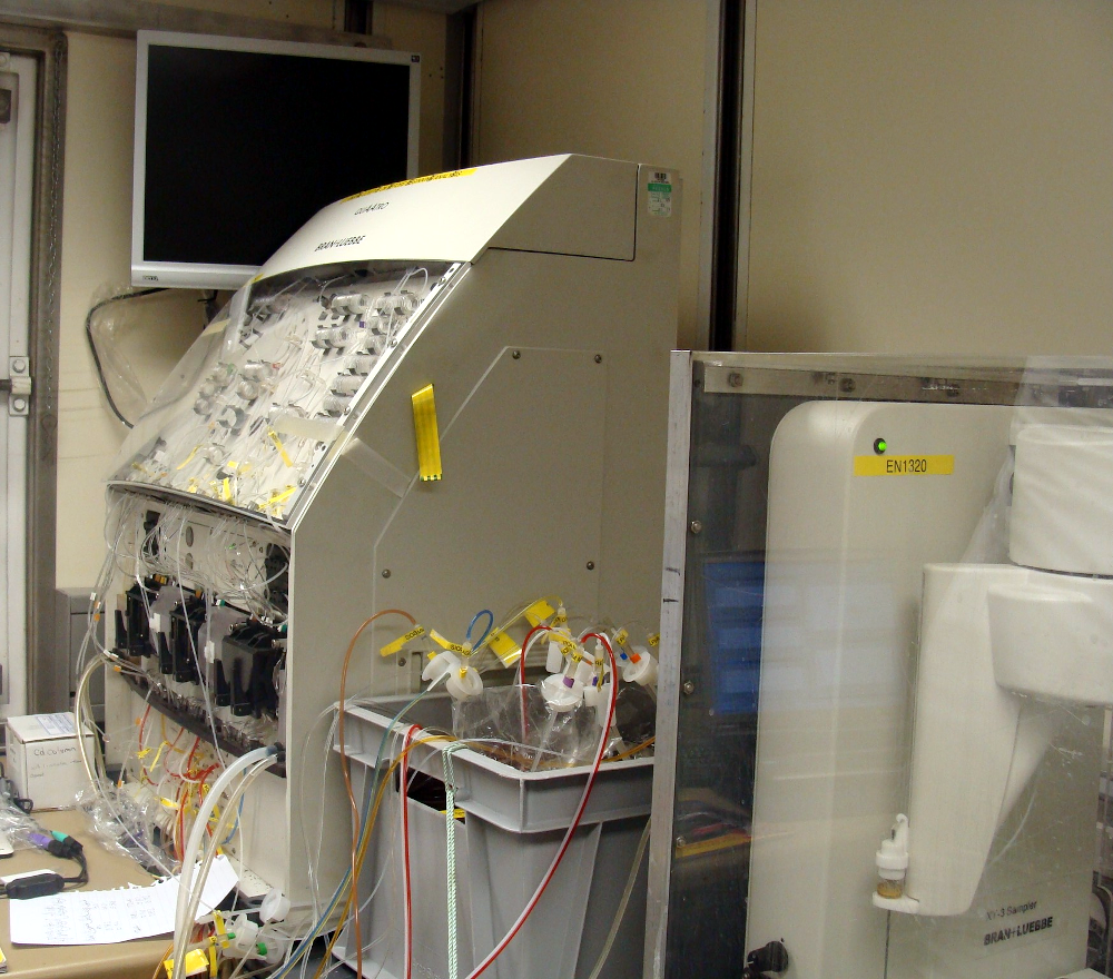
Figure 1: Winter Nutrient Analysis in the containerised laboratory on MRV Scotia

The availability of inorganic nutrients is essential for the growth and distribution of primary producers such as phytoplankton. Growth of phytoplankton can be limited by the supply of nutrients, in particular dissolved inorganic nitrogen (DIN) (of which nitrate is most abundant), dissolved inorganic phosphorous (DIP) (mainly as phosphate) and dissolved silicate (DSi).

Anthropogenic inputs of nitrogen and phosphorus to coastal and offshore areas from sources such as agriculture and industrial waste disposal may result in elevated nutrient concentrations.

Eutrophication in the marine environment is the excessive growth of phytoplankton in response to this elevation of nutrient concentrations resulting in undesirable disturbance in the marine ecosystem.

The Marine Strategy Framework Directive (MSFD) sets out eleven qualitative descriptors against which Good Environmental Status (GES) should be assessed. Descriptor 5 (Eutrophication) states that ‘Human-induced eutrophication is minimised, especially adverse effects thereof, such as losses in biodiversity, ecosystem degradation, harmful algal blooms and oxygen deficiency in bottom waters’.

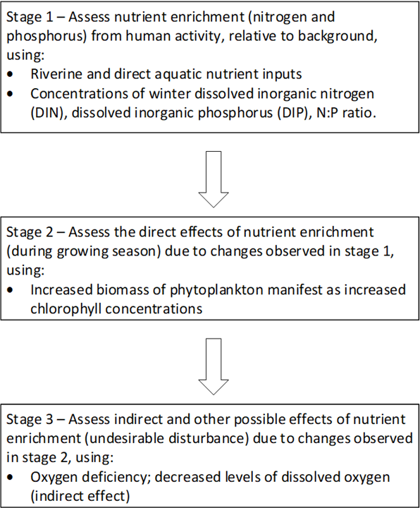
One of the common indicators for MSFD Descriptor 5 is ‘Winter nutrient concentrations’. The assessment of eutrophication within the Scottish Marine Assessment is split into indicators of nutrient enrichment, direct nutrient effects and indirect nutrient effects as per the OSPAR and MSFD eutrophication assessment methodology (Figure a, (OSPAR, 2017)).

Eutrophication is a problem if there is evidence of nutrient enrichment (Stage 1; inputs & winter nutrients), direct effects of nutrient enrichment (Stage 2; elevated chlorophyll concentration, increased blooms) and indirect effects of nutrient enrichment (Stage 3; oxygen deficiency, biomass changes).

This indicator assesses winter nutrient concentrations (Stage 1; nutrient enrichment), defined as the period November – February inclusive, in the Scottish marine environment and does not consider the other stages, which will be considered in the overall assessment of Eutrophication.

Figure a: The three stages of eutrophication assessment. The criteria Nitrogen/ Phosphorus ratios are not applied in UK waters but used as additional evidence.

Eutrophication monitoring is undertaken in Scottish waters as part of the Water Framework Directive (WFD) by SEPA and MSFD (SEPA and MSS). Nutrient (MSS and SEPA), chlorophyll and dissolved oxygen (SEPA only) data for marine waters are submitted annually to the UK Marine Environment Monitoring and Assessment National (MERMAN) database. For this assessment only the MSS winter nutrient data submitted to MERMAN have been used.

Description of data

Water samples were collected in coastal and offshore areas on MSS’s annual (January) Clean Seas Environment Monitoring Programme (CSEMP) cruise between 2007 and 2019 on the hour and every 15-30 minutes thereafter. Samples were analysed for nutrients (total oxidised nitrogen (TOxN), phosphate (DIP), silicate (DSi) and ammonia).

Nutrient data for marine waters were submitted annually to the UK Marine Environment Monitoring and Assessment National (MERMAN) database, along with associated Quality Control (QC) data held at the UK Datacentre (BODC, (MERMAN, 2019)). The data were automatically validated before they were loaded into the database against set criteria. If there was appropriate good quality QC information, then the data passed the data filter. If not, then data were still accepted into the database but not used in any assessment. These data were subsequently submitted to ICES environmental database (September of the same year). Only data that passed the data filter were forwarded to ICES.

SEPA’s WFD data and MSS’s coastal and offshore data on winter nutrients, chlorophyll-a, phytoplankton and dissolved oxygen contribute to the OSPAR Common Procedure (OSPAR, 2016). The OSPAR Eutrophication Strategy requires Contracting Parties to provide data to assess the eutrophication status of their marine waters as part of the Common Procedure.

The causative factors (nutrient inputs and winter nutrient concentrations) are used to highlight areas where further monitoring is required to assess the impact on the ecology (accelerated growth of phytoplankton and macroalgae) leading to an undesirable disturbance (excessive organic inputs leading to low dissolved oxygen and kills of fish and benthos).The OSPAR Comprehensive Procedure requires water bodies to be classified as Non-Problem Areas (NPA), Potential Problem Areas (PPA) or Problem Areas (PA), depending on their eutrophication status. The latest OSPAR assessment can be found in OSPAR (2016).

Status and trends of nutrients are assessed and summarised for each Scottish Marine Region (SMR) where there are sufficient data. This involves utilising soap-film smoother Generalised Additive Models and assessing against the criteria used in OSPAR, WFD and MSFD eutrophication assessments (OSPAR, 2016 & 2017).

MSS comply with ISO 17025 and are UKAS accredited and participate in the QUASIMEME proficiency testing scheme for nutrients and chlorophyll analysis.

Winter Nutrient Concentration Assessment and Geographical Scale

OSPAR Ecological Quality Objectives (EcoQOs) for nutrient enrichment in the UK have been developed for dissolved inorganic nitrogen (DIN; the sum of the concentration of TOxN (nitrate plus nitrite) and ammonia) and the ratios DIN to DIP in coastal waters (defined as having salinities between 30.0 and 34.5) and offshore waters (salinities greater than 34.5).

The elevated concentrations are defined as 50% above the background concentration for DIN (OSPAR, 2017, Table a). The coastal criteria require DIN concentrations to be normalised to a salinity of 32.0 by assuming conservative mixing along a constant gradient with a zero salinity endpoint of 42 μM (Devlin, Painting & Best, 2007). This freshwater value was determined in the river Leven (Cumbria) and was assumed to be representative of a relatively unpolluted rural river system. OSPAR assessment criteria refer to DIN (TOxN plus ammonia), whereas only TOxN has been modelled in this assessment.

The ammonia contribution to DIN in offshore water is considered negligible in Scottish waters, with little difference between DIN and TOxN concentrations (Smith et al., 2014).

The elevated DIN/DIP (N/P) ratio set for UK waters is 24 (OSPAR, 2017). The UK have not set thresholds for winter DIP because nitrogen is defined as the limiting nutrient in UK waters and therefore in this assessment DIP has been provided for information only.

Table a: Background and assessment concentration levels for winter DIN concentrations, DIN/DIP (N/P) and DIN/DSi (N/S) ratios set for UK coastal and offshore waters. Coastal waters are classed as having a salinity of 30 - 34.5 and offshore waters >34.5.
Parameter	Background	Elevated
DIN (Offshore)	10 µM	15 µM
DIN (Coastal)	12 µM	18 µM
N/P	16	24
N/S	1	2

The area of the assessment is based on 11 SMRs. The SMRs encompass both coastal (salinity of 30 - 34.5 ) and offshore (salinity >34.5) waters, therefore different assessment criteria apply within them. There is limited availability of data to permit assessments in all Offshore Marine Regions (OMRs) and this assessment has focussed on the SMRs.

Data Preparation

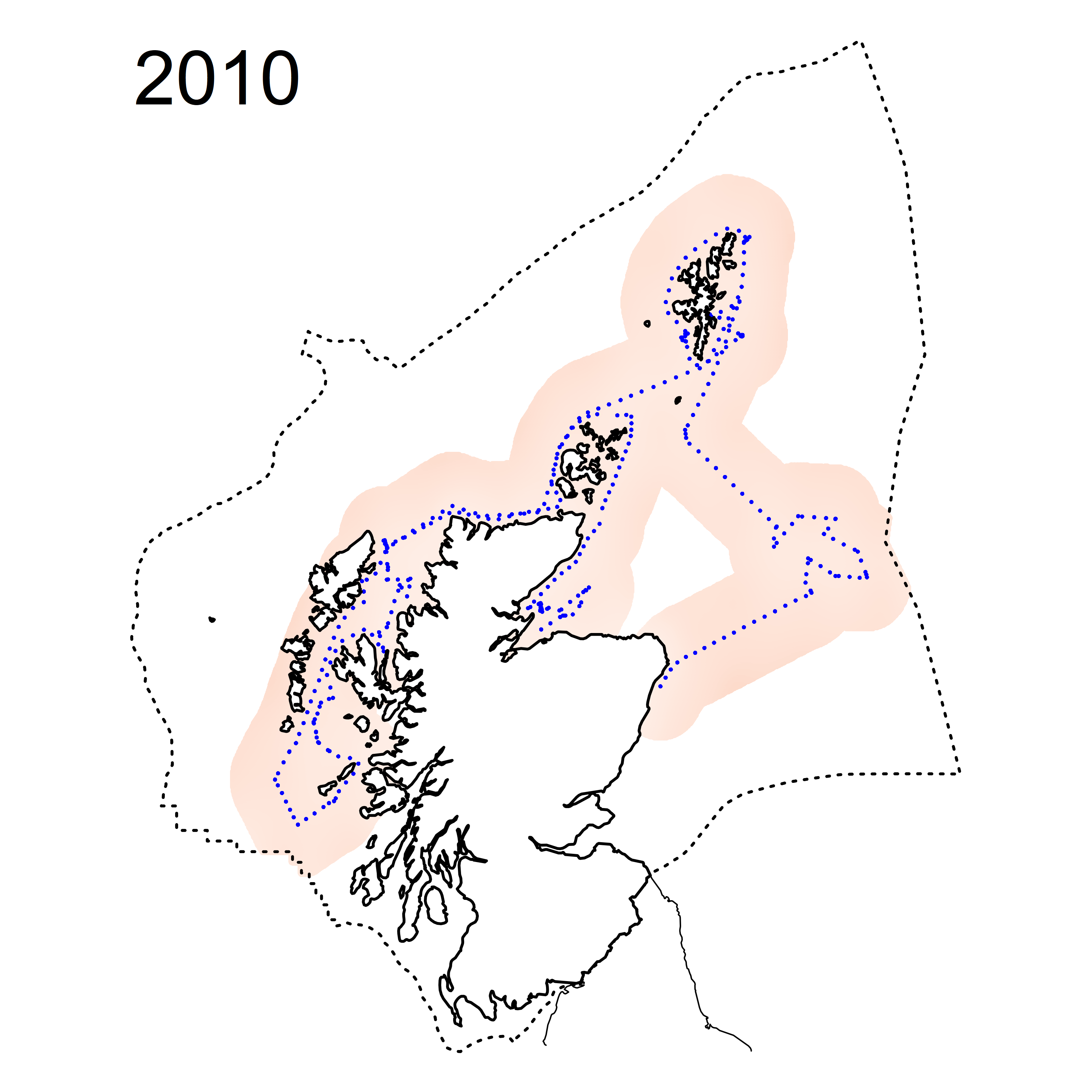
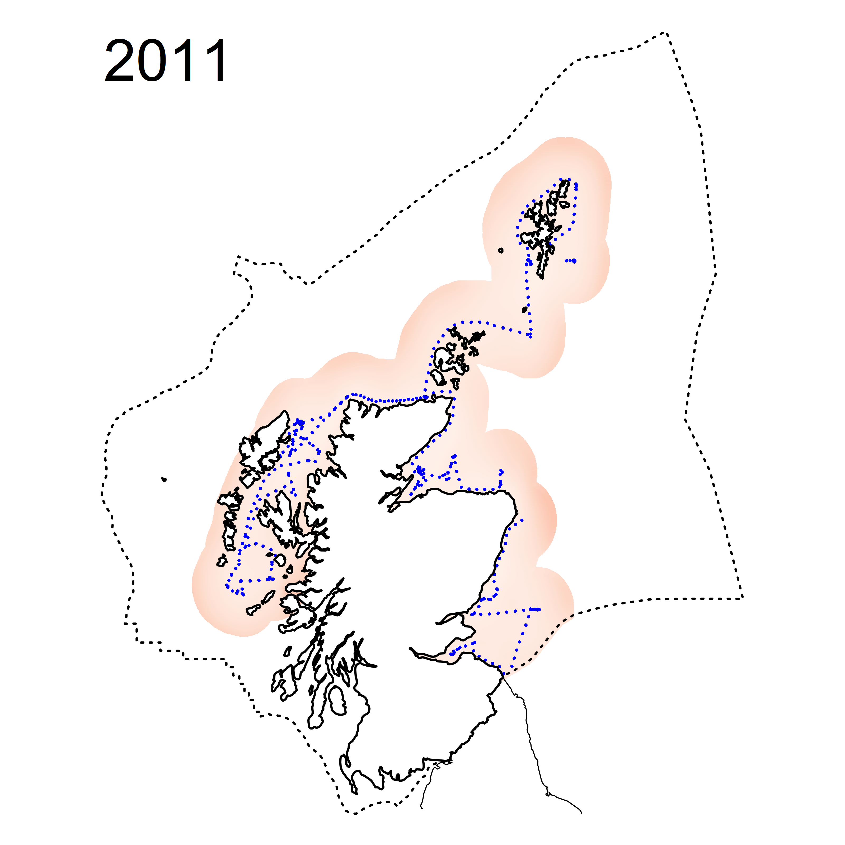
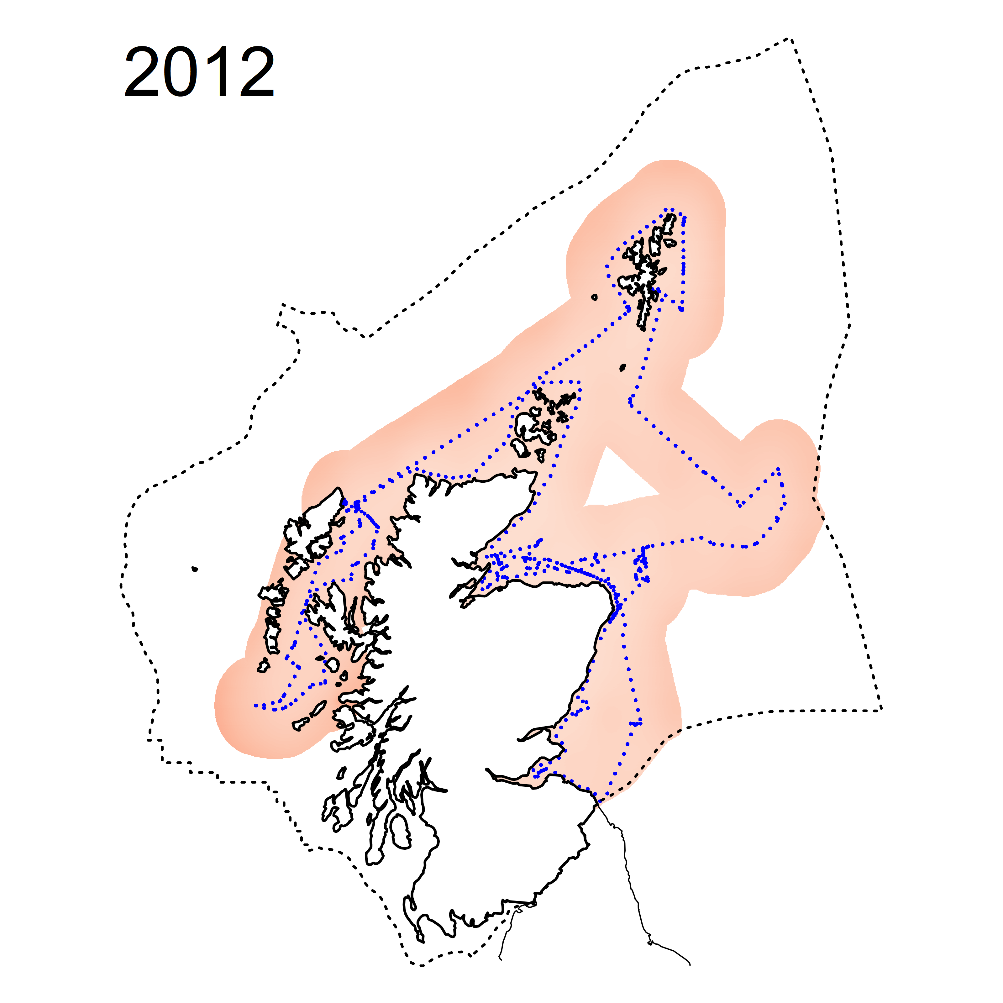
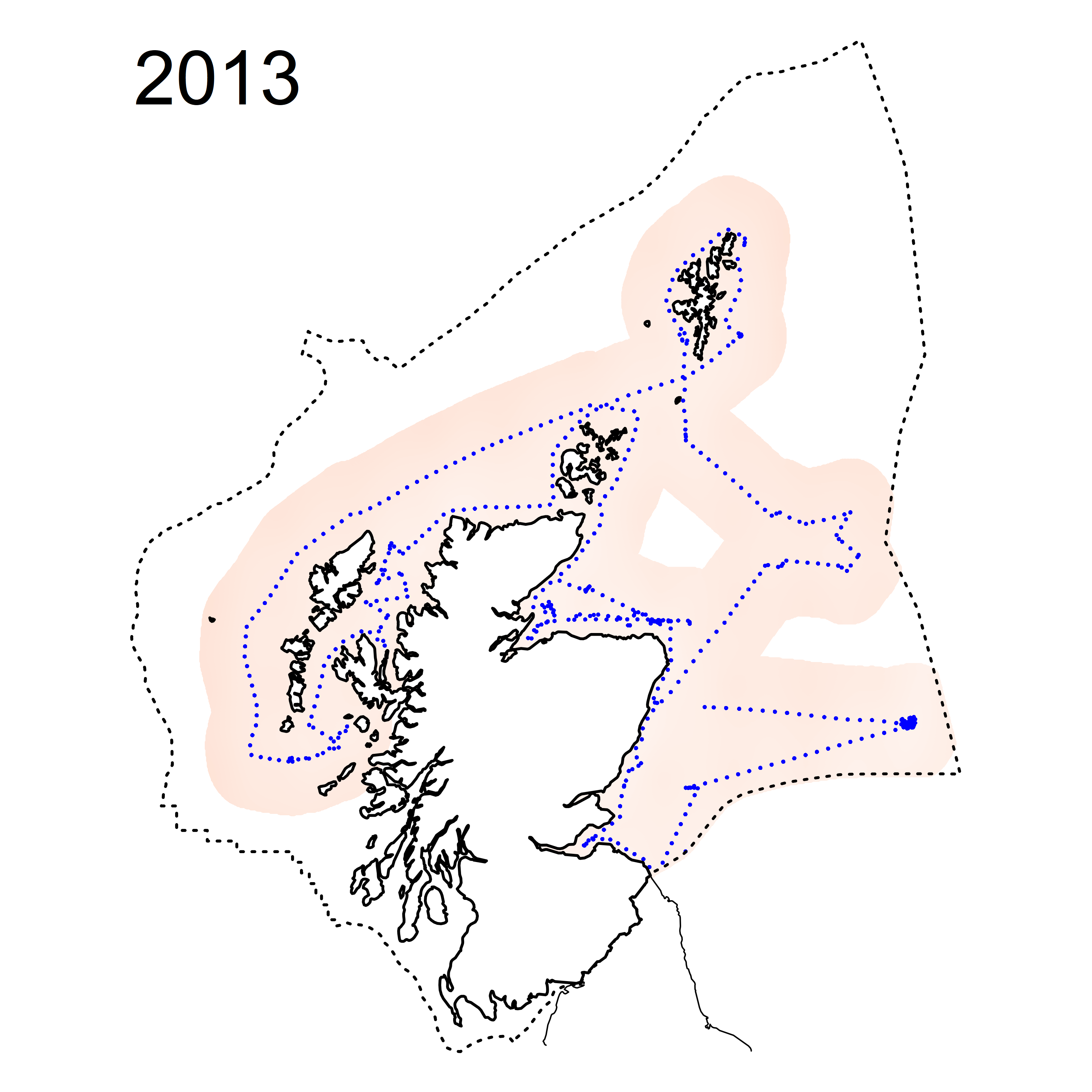
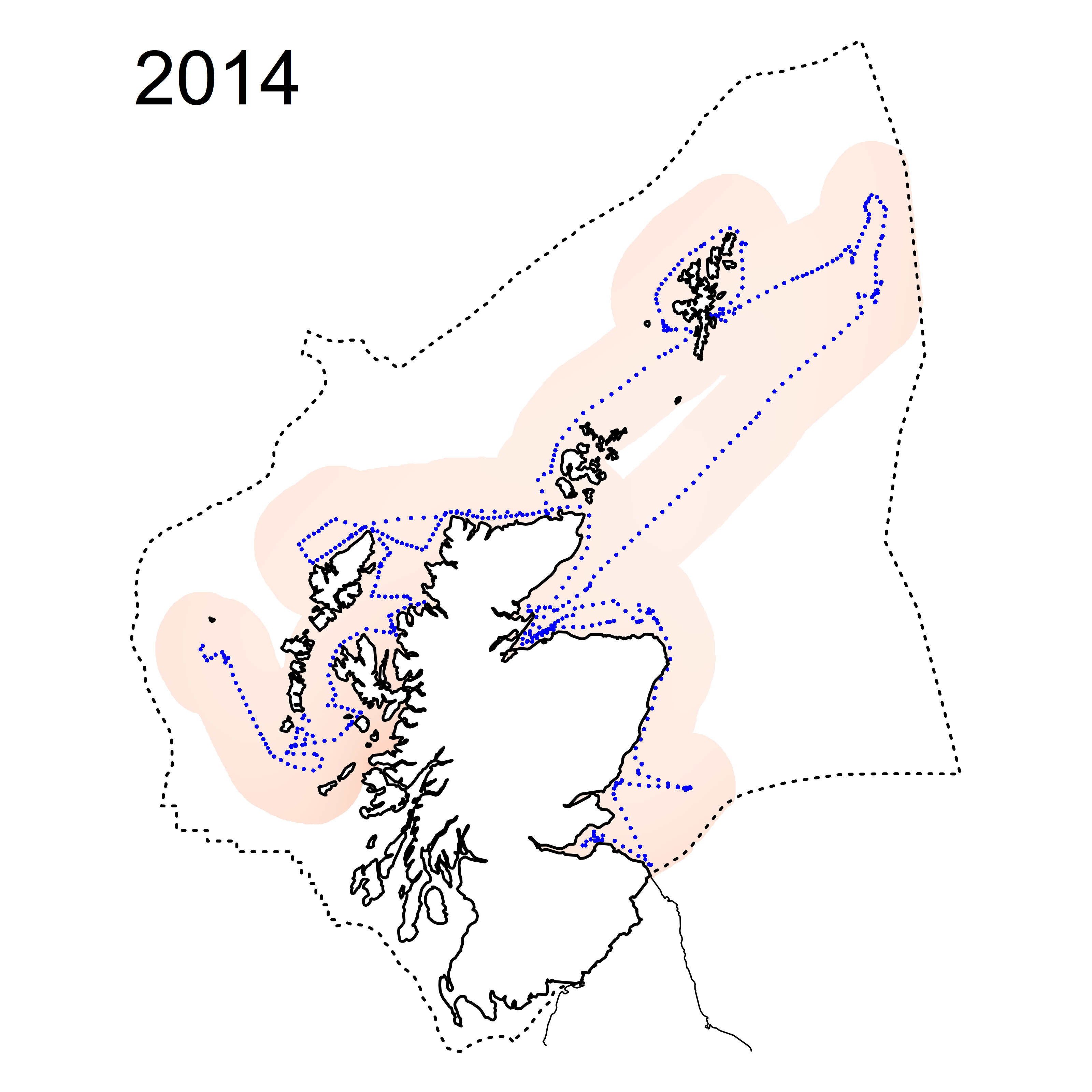
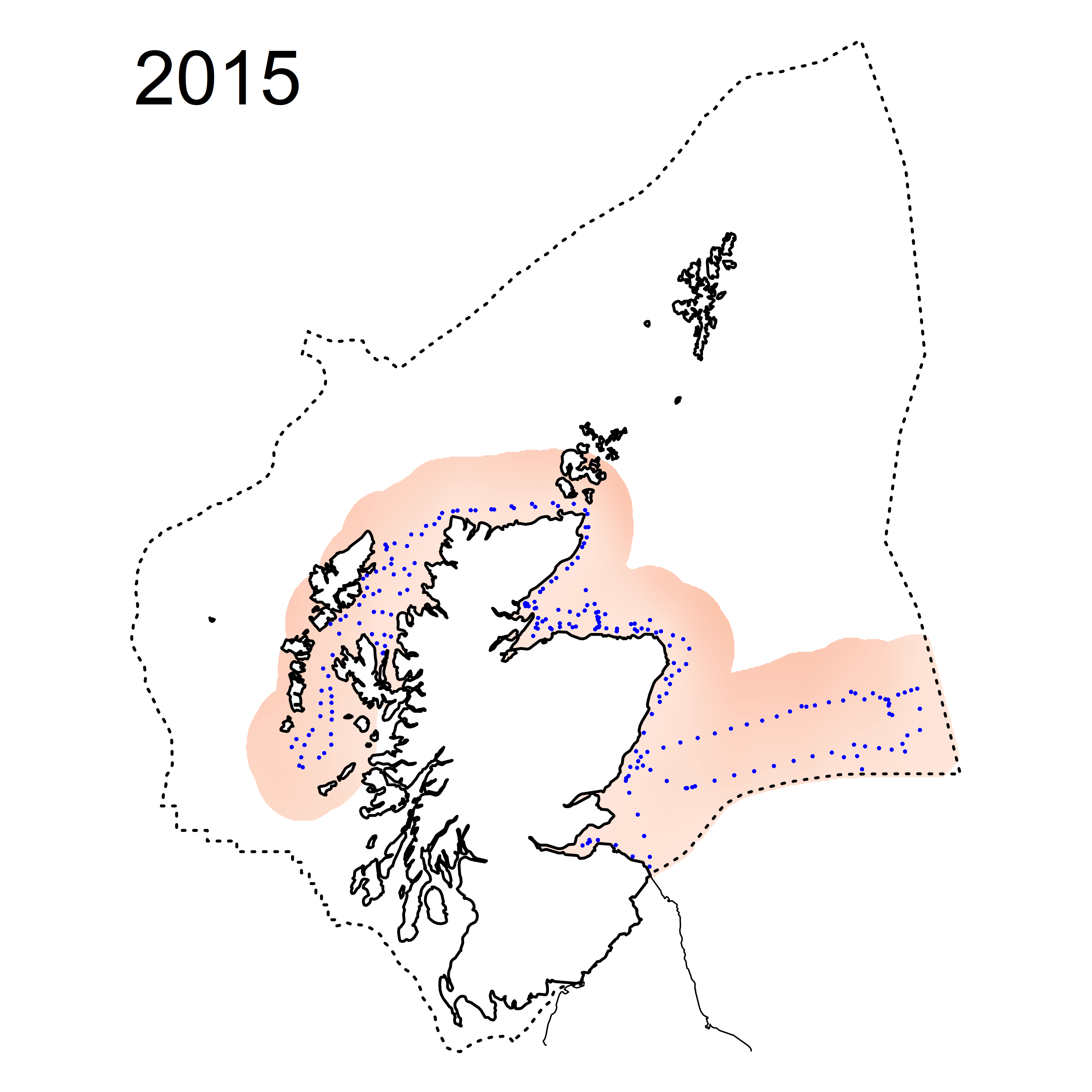
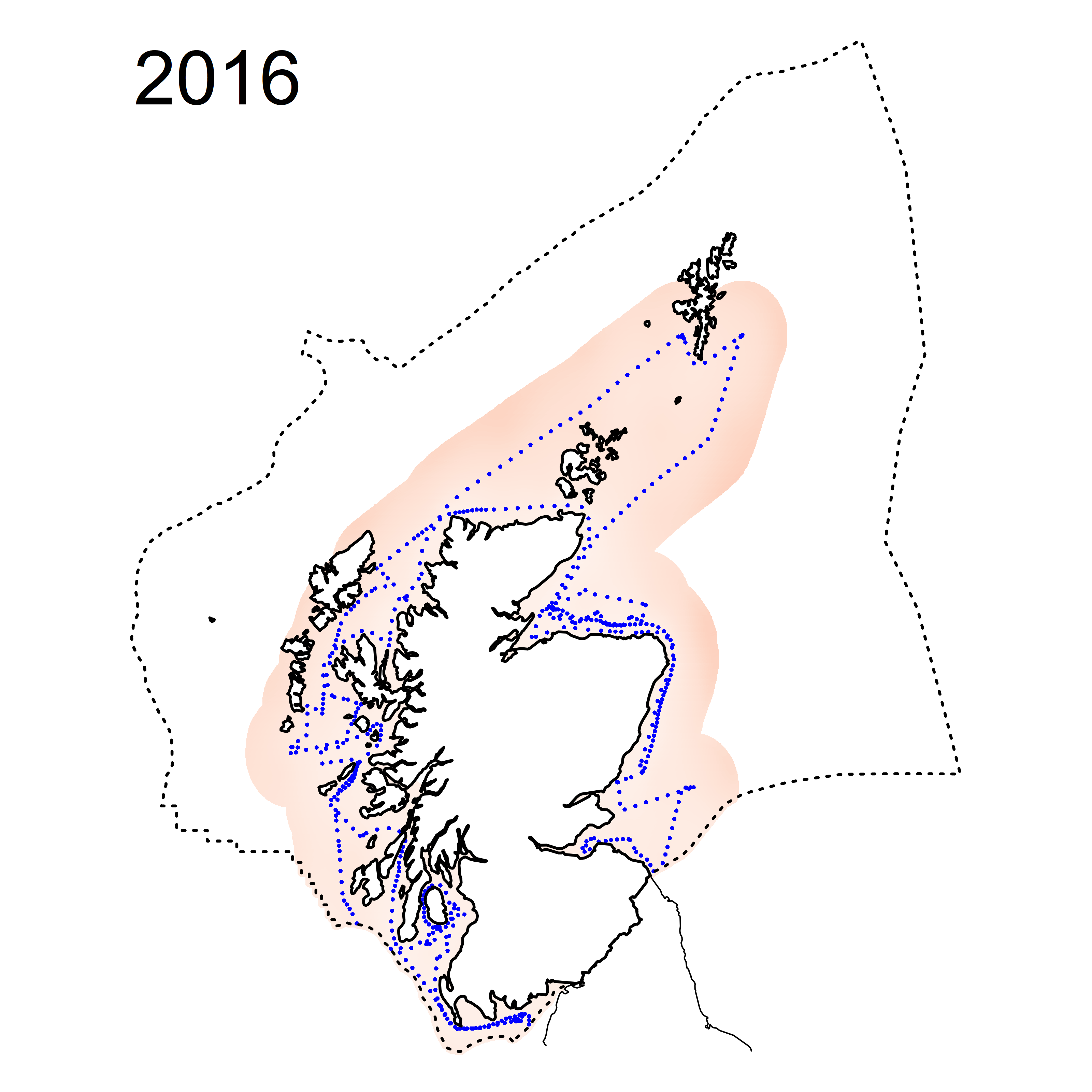
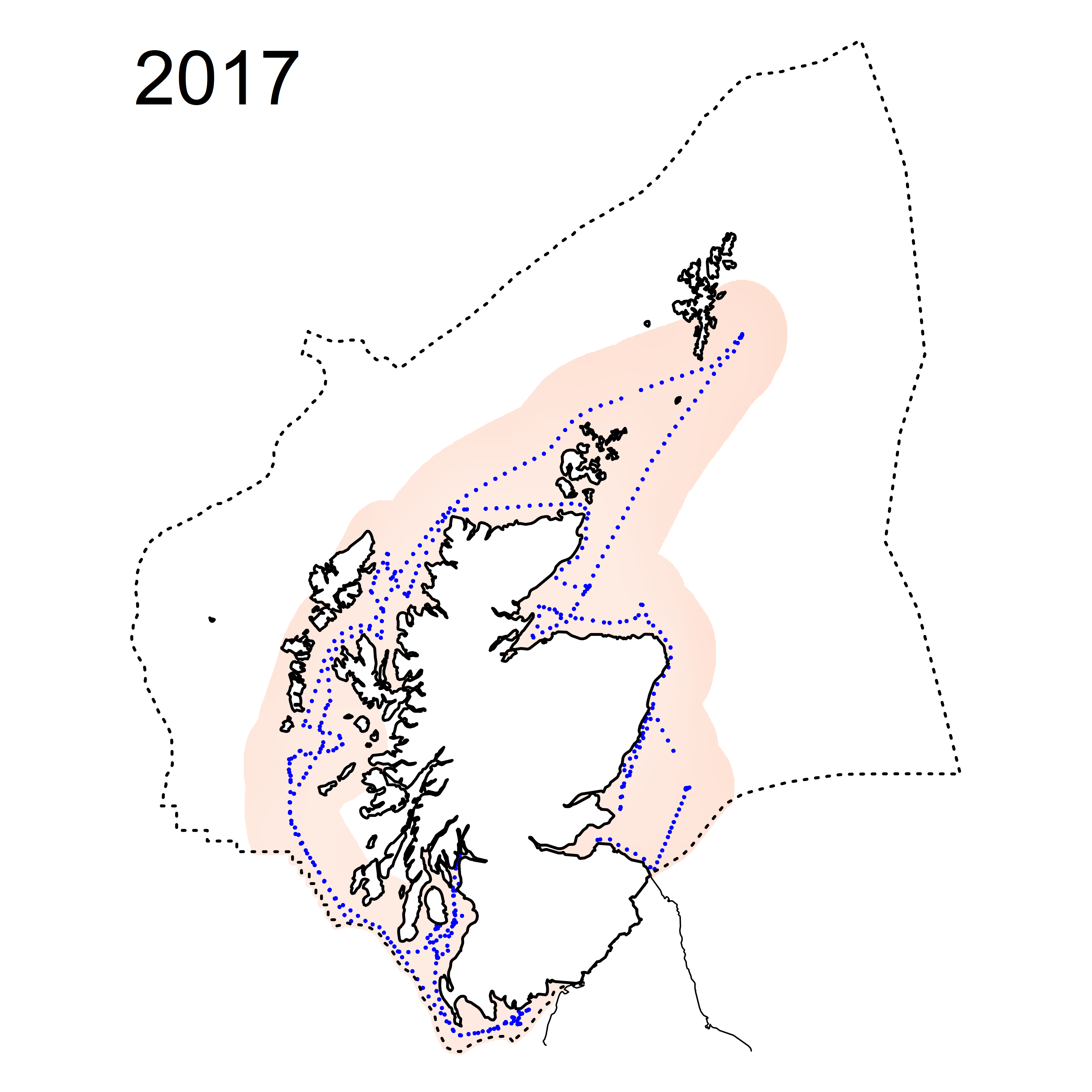
Data from MSS CSEMP MERMAN submissions were assembled and prepared for analysis within the R statistical environment, version 3.5.2 (R Core Team, 2018). All data are within an area incorporating the Charting Progress 2 biogeographic regions of Irish Sea, Minches and Western Scotland, Northern North Sea and Scottish Continental Shelf (United Kingdom Marine Monitoring and Assessment Strategy, 2010) (Figure 2) within the Scottish Zone. Data quality checks were undertaken and occasional errors corrected or deleted.

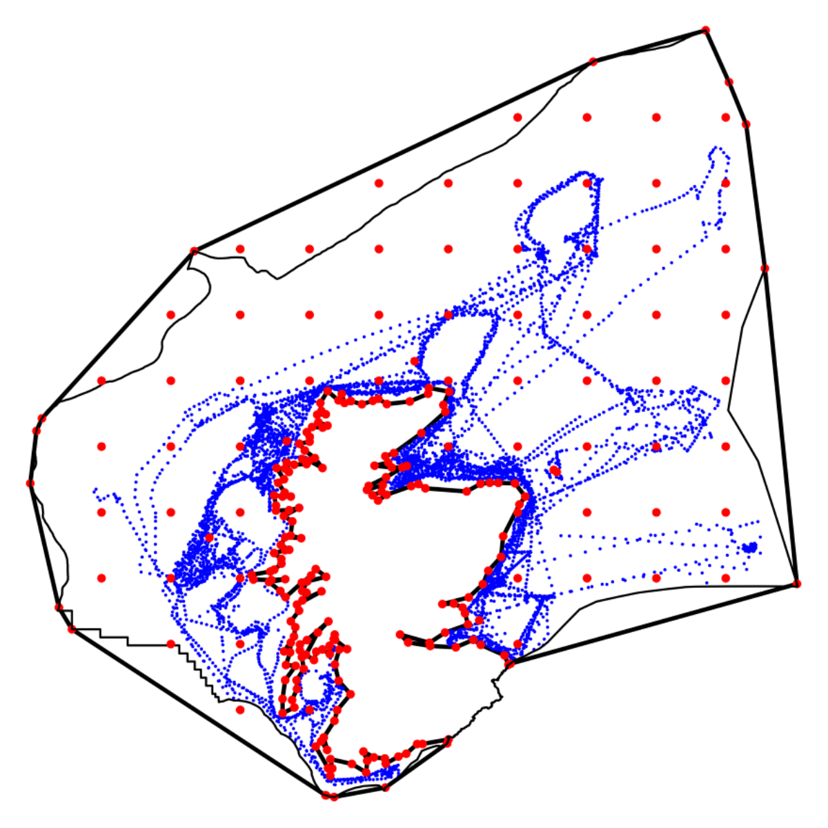Figure b: Isotropic statistical model set-up and sampling locations.

Figure 2: Isotropic statistical model set-up and sampling locations. The modelling area is denoted by a thick continuous boundary line, the relevant part of the Scottish Zone by a thin continuous boundary line, sampling locations by small blue points, and ‘knots’ around which the smoothers are based by large red points.

Statistical modelling

The analyses describe spatial distributions and between-year temporal changes for the nutrients of total oxidised nitrogen normalised for salinity (TOxN), dissolved inorganic phosphorus (DIP), dissolved silicate (DSi), the ratio of TOxN to DIP (N:P), and the ratio of TOxN to DSi (N:S). The spatial variation of nutrients was modelled on an annual basis utilising soap-film smoother Generalized Additive Models (Wood, Bravington & Hedley, 2008). A first smoother estimates nutrient quantities based around ‘knots’ along an outer boundary and a second smoother estimates distortions away from these based around ‘knots’ within the boundary. This approach avoids smoothing nutrient quantities across the land-mass. The statistical methodology has been used for this purpose previously (Smith et al., 2014) but has been implemented differently for this assessment.

Boundary and knot positions, which were converted from coordinates to isotropic grid references for analysis, are presented (Figure 2). Statistical modelling involved fitting each nutrient to explanatory variables including the boundary smooth and within-boundary smooth for each individual year. The statistical model comprised:

$\ln [E (y_{i j k})] = β_{0} + f (x_{i} x_{j}) + u_{k}$

where y_ijk = nutrient quantities TOxN, DIP, DSi, N:P or N:S sampled at grid reference i, j and laboratory analytical batch k - values of y_ijk are assumed to follow a Gamma error distribution incorporating a lag 1 autoregressive correlation modelling dependence on the previously collected sample; β₀ = estimated fixed effect intercept; f(xi,xj) = estimated boundary and within-boundary soap-film smoothers; and u_k = random effect for laboratory analytical batch k. Estimates of β₀, f and u_k were calculated by penalised quasi-likelihood within the R supplementary package mgcv 1.8-27 (Wood, 2017).

The primary differences with the approach of Smith et al. (2014) is that this analysis utilises isotropic distances rather than coordinates, and models individual years rather than groups of years. Modelled nutrient quantities for each year and their coefficients of variation at 1 km intervals were calculated and utilised for two plots comprising:

annual modelled nutrient quantities within 54 km of sampling positions; this corresponds to 4% of the maximum north-south distance, less than that used by Smith et al. (2014);
a summary of the weighted mean modelled values for the winters 2016/17 to 2018/19 inclusive; weights comprise the proportion of the inverse of the variance of the three annual modelled values for locations included in the relevant annual plots.

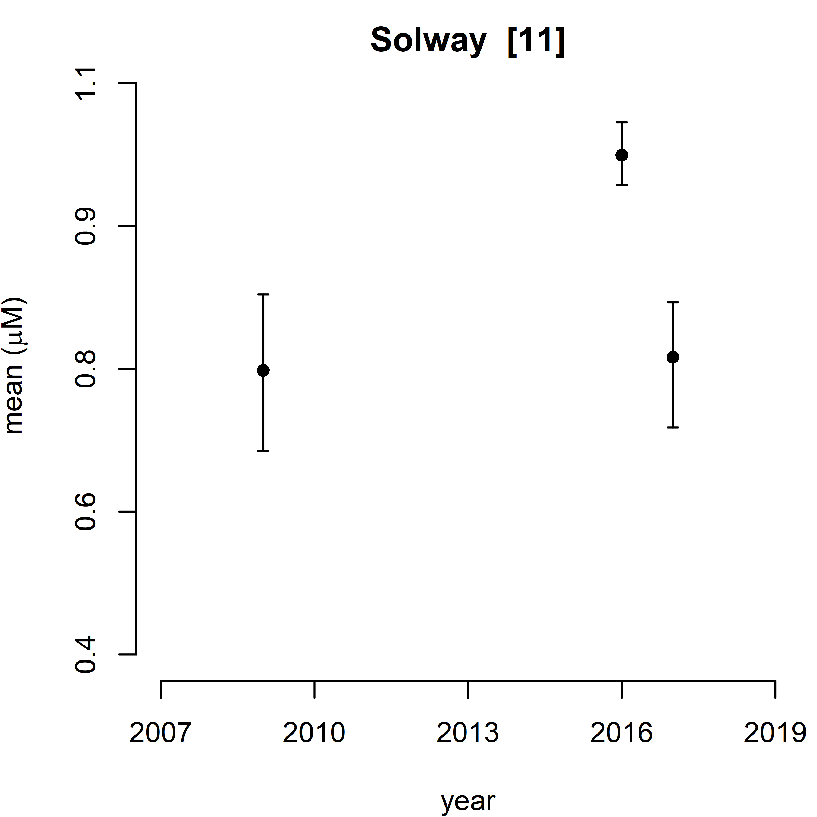
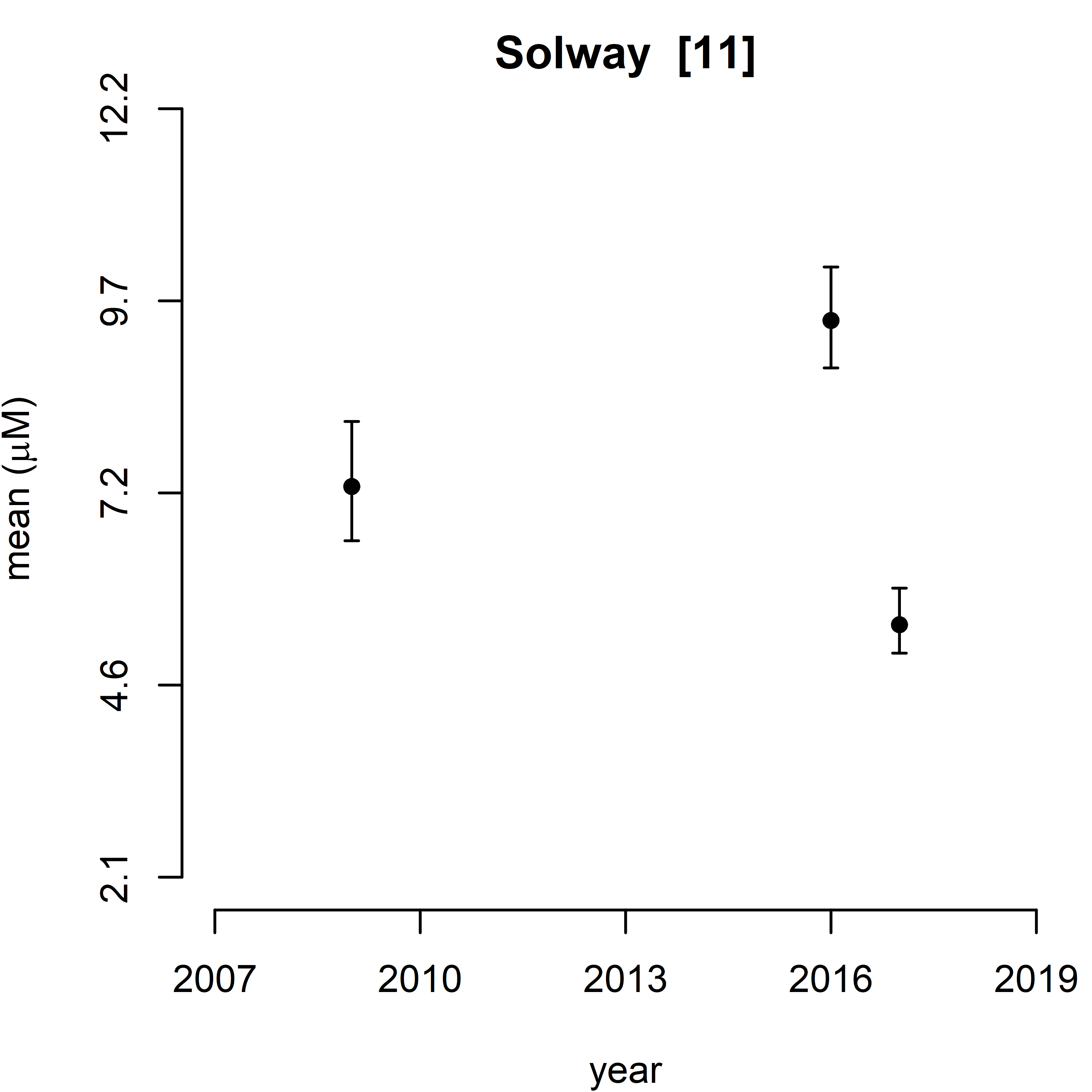
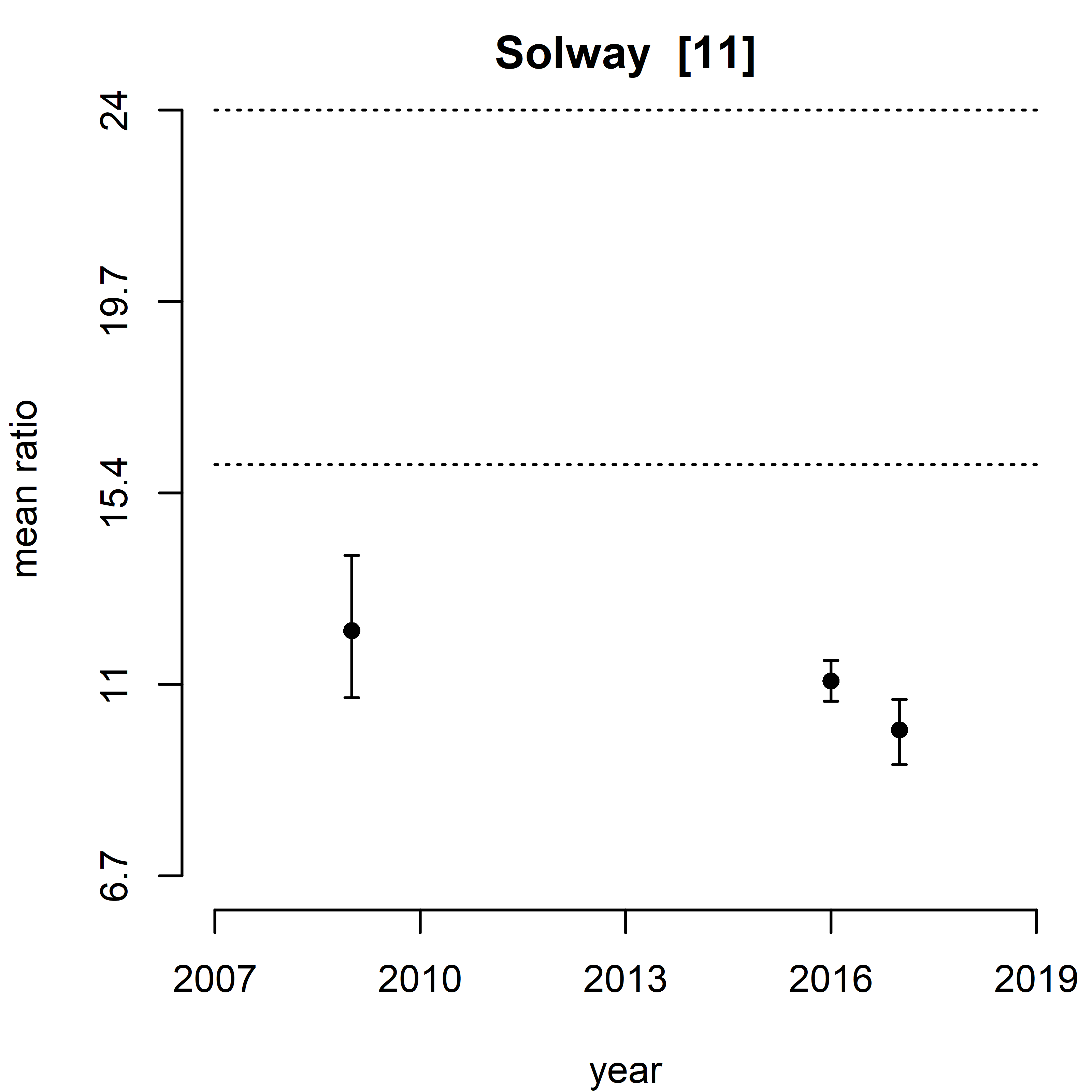
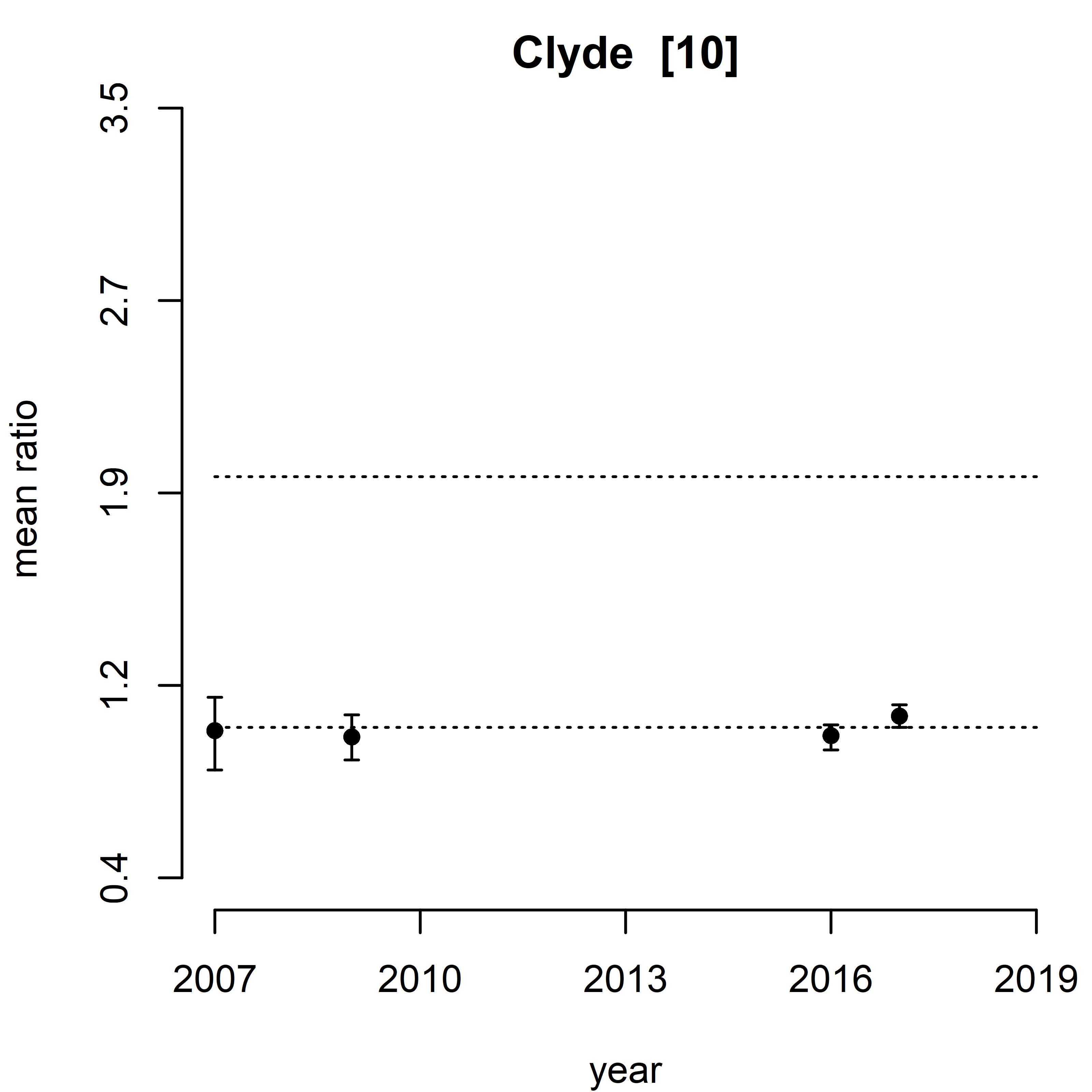
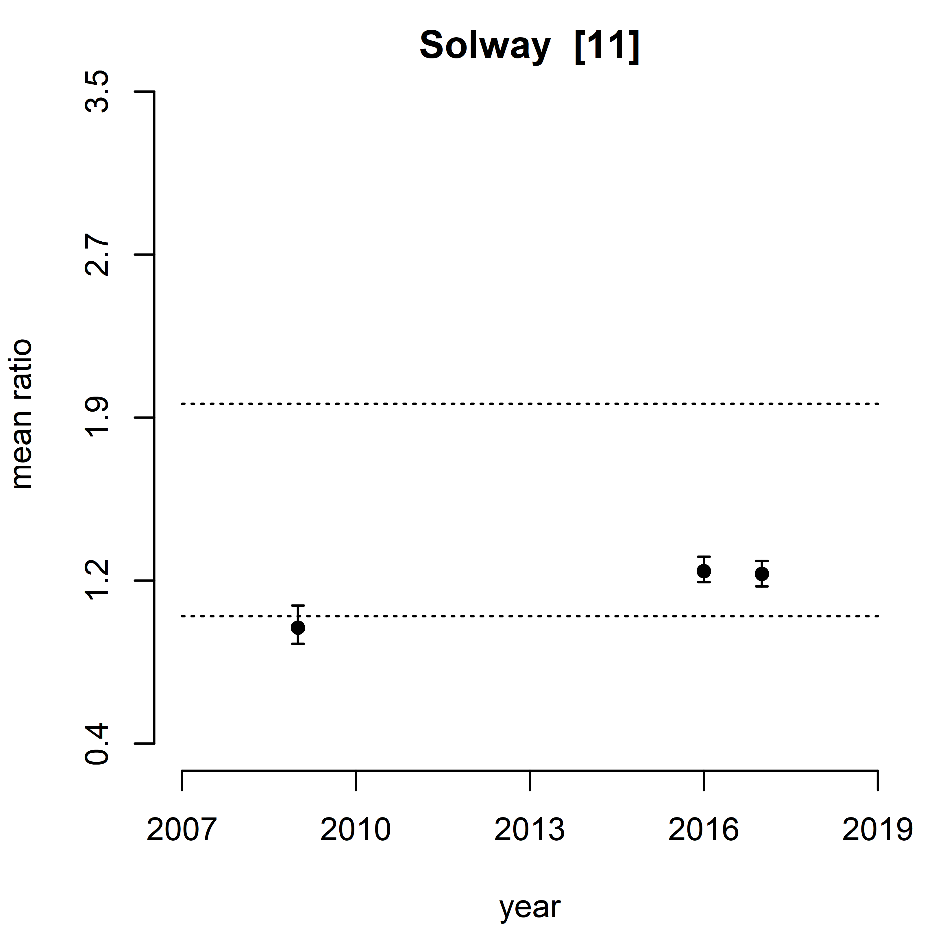
Annual means and percentile 95% confidence intervals were estimated for the relevant parts of 11 SMRs if the coverage of modelled values was regarded as satisfactory. Mean values were only estimated for an SMR when the predicted values covered at least 80% of the relevant area. For example mean values for only 2009, 2016 & 2017 are presented for the Solway because the predicted values in other years covered < 80% of the Solway SMR because of sampling. The 95% confidence intervals were estimated using a parametric bootstrap (Efron, 1979) utilising the lpmatrix option of the gamm predict function.

Temporal trends for the SMR from winter 2007 to 2019 were estimated using an additive model. The model compromised:

$Y_{t} = β_{0} + f_{t} + u_{t} + ε_{t}$

where y_t = the annual mean nutrient (TOxN, DIP, DSi, N:P or N:S) quantity in year t assuming error variation ~N(0,σ_t²); β₀ = estimated fixed effect intercept; f_t = estimated function comprising a smoother limited to 3 degrees of freedom over years t; u_t = estimated random effect of year t assuming ~N(0,σ_t²); ε_i = residual variation; σ_t²= variance of the error term x 4. While the potential values of y_t are constrained by a minimum of 0, the lower confidence intervals which all exceeded zero are consistent with an assumption of normality. The model was fitted by residual maximum likelihood (Patterson & Thompson, 1971). Temporal plots for each SMR were generated.

Values of p are interpreted as a level of support for ‘no-effect’ and are regarded as ‘statistically significant’, indicating a lack of support for the null hypothesis, if no greater than 0.050.

Results

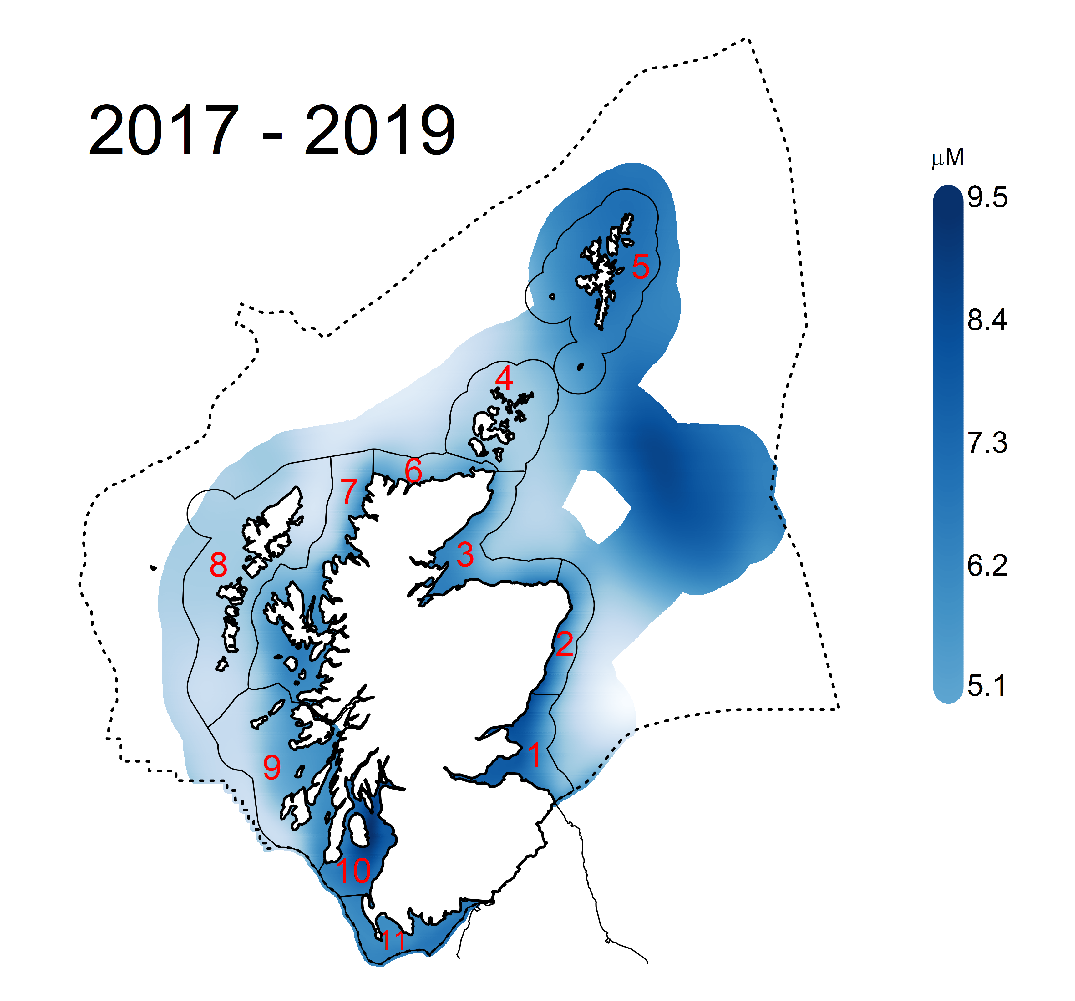
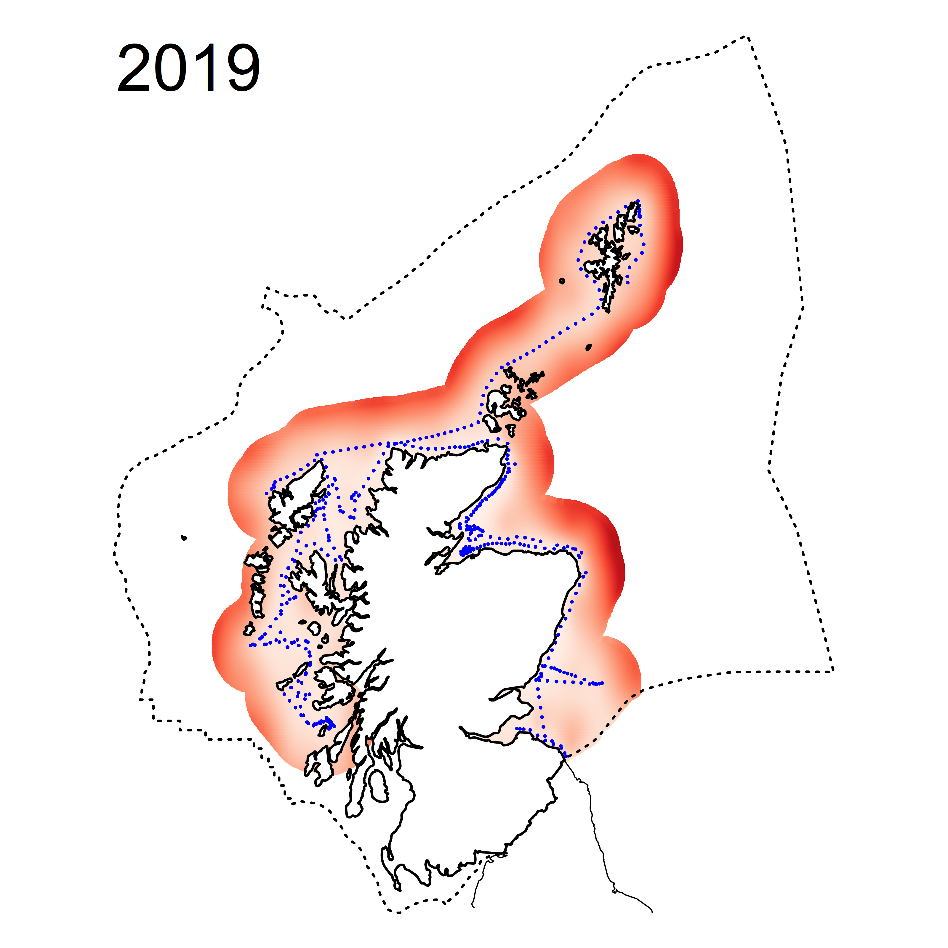
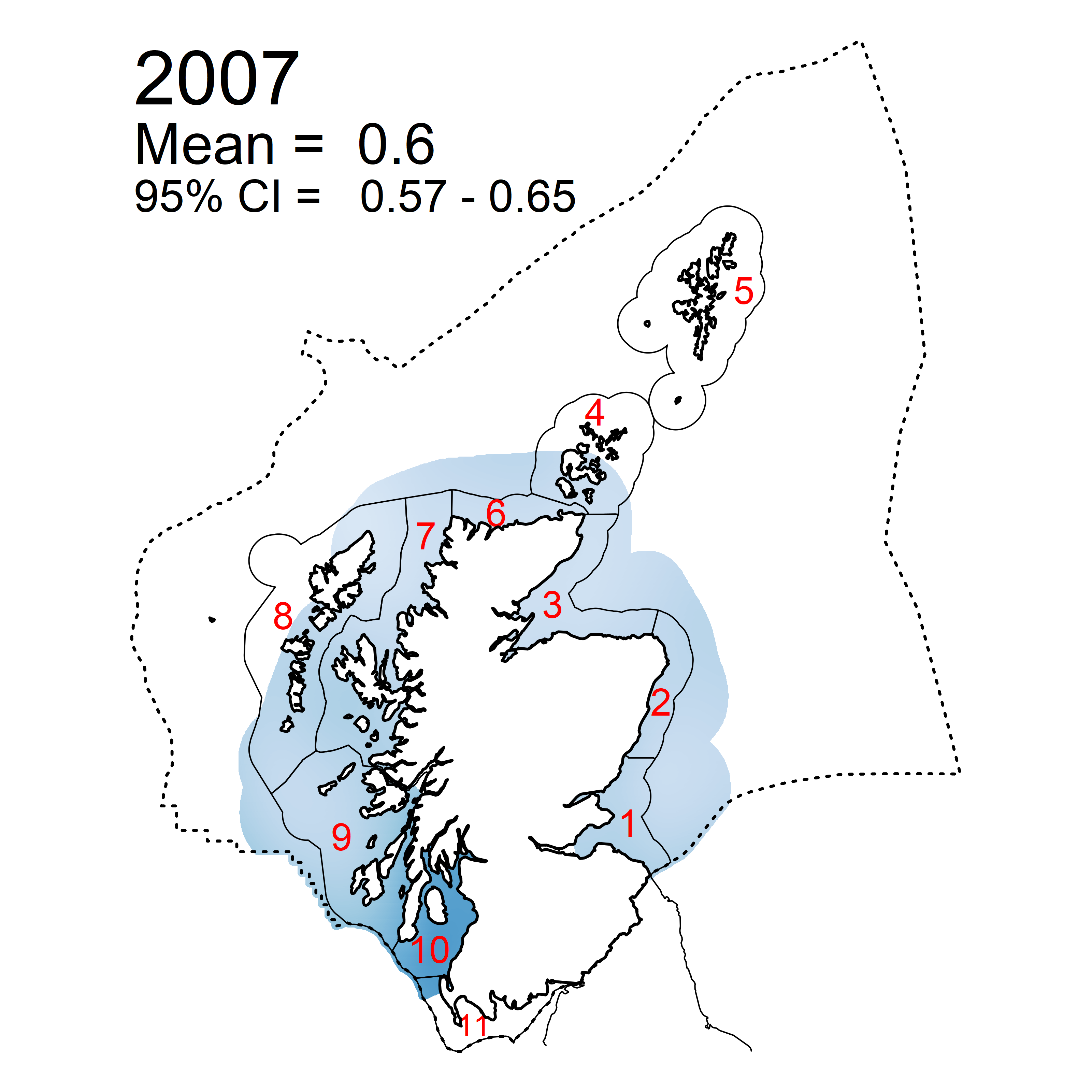
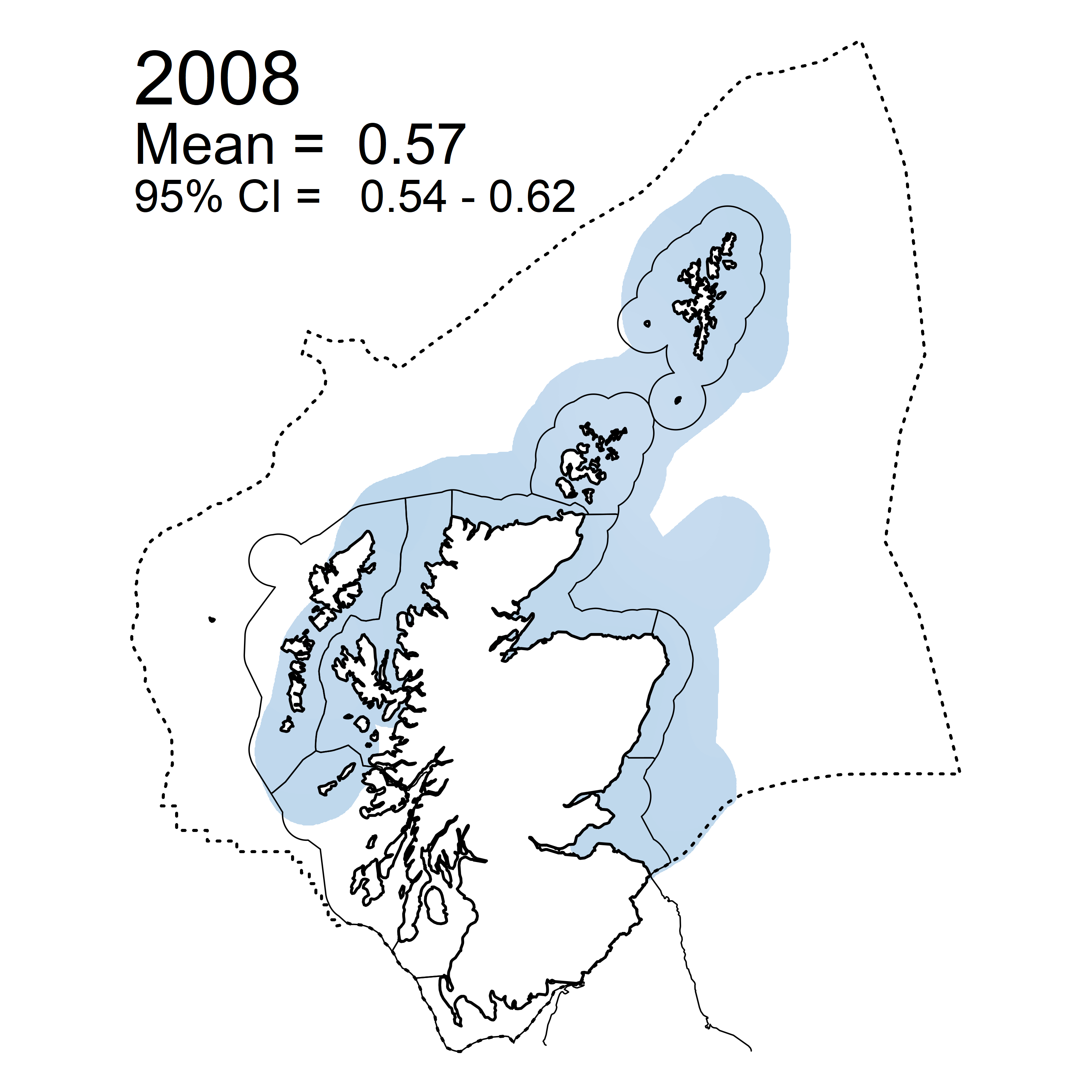
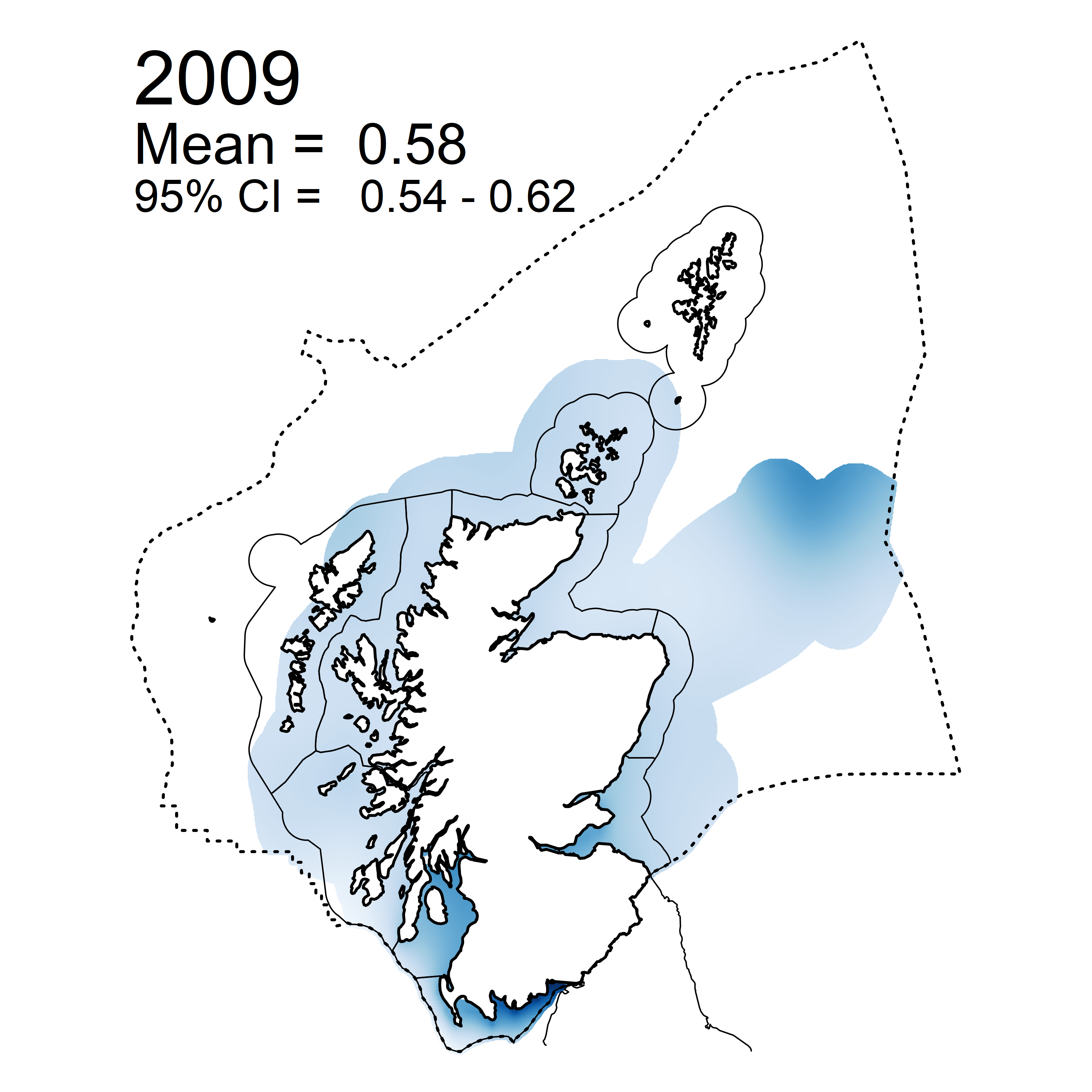
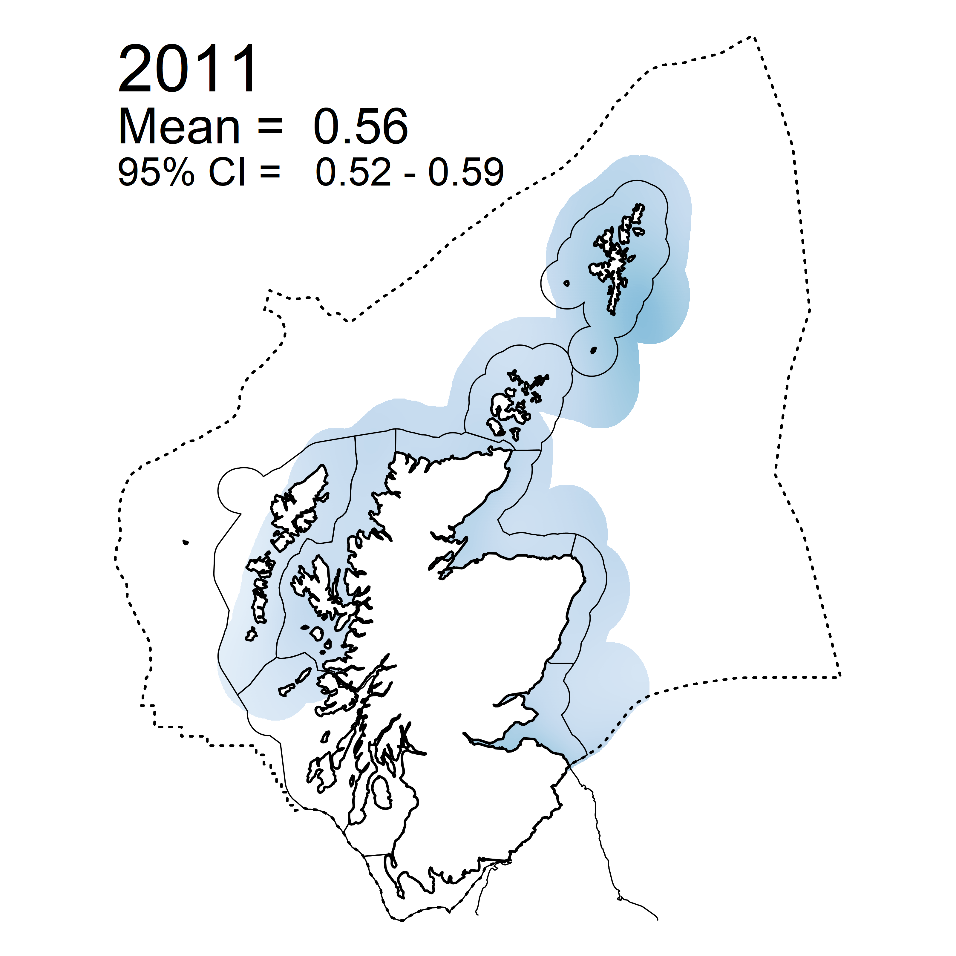
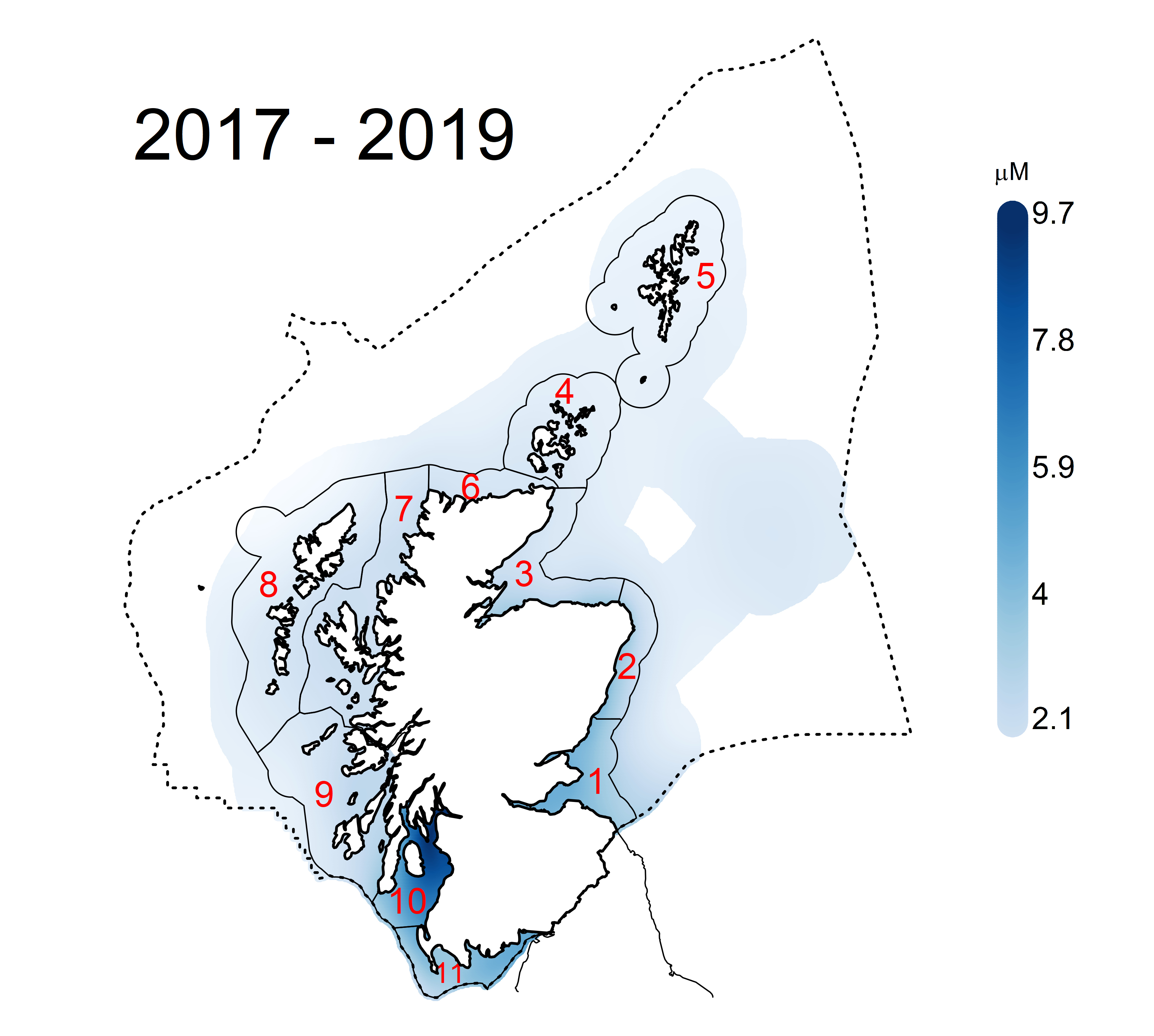
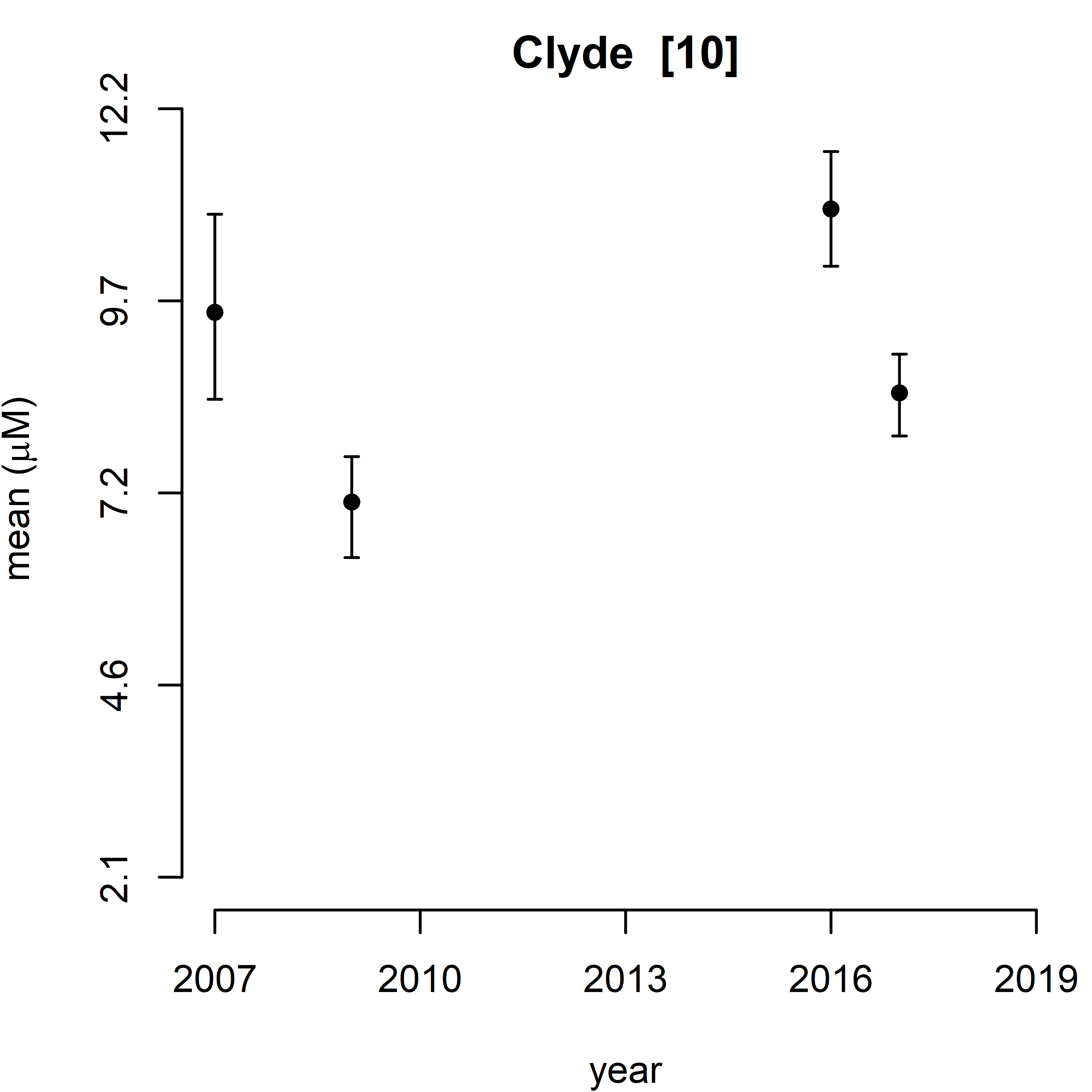
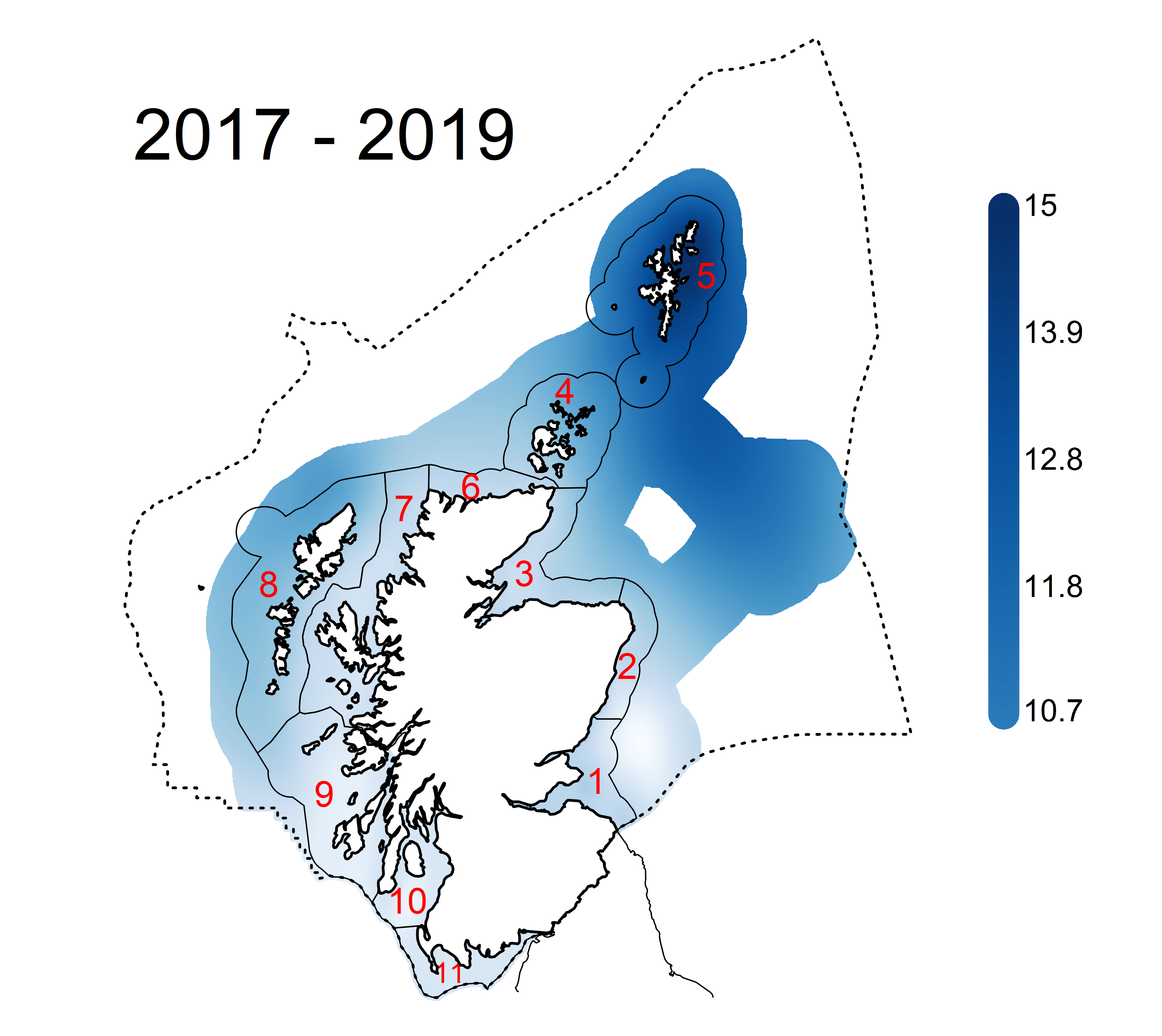
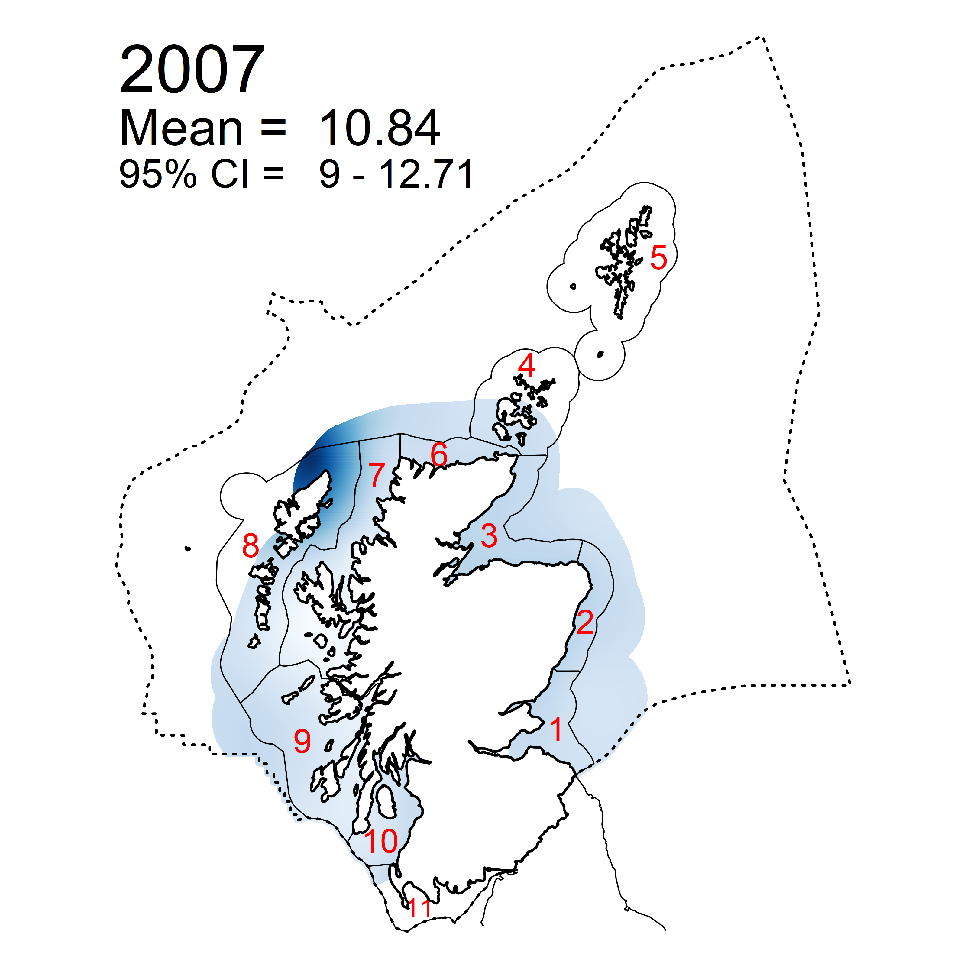
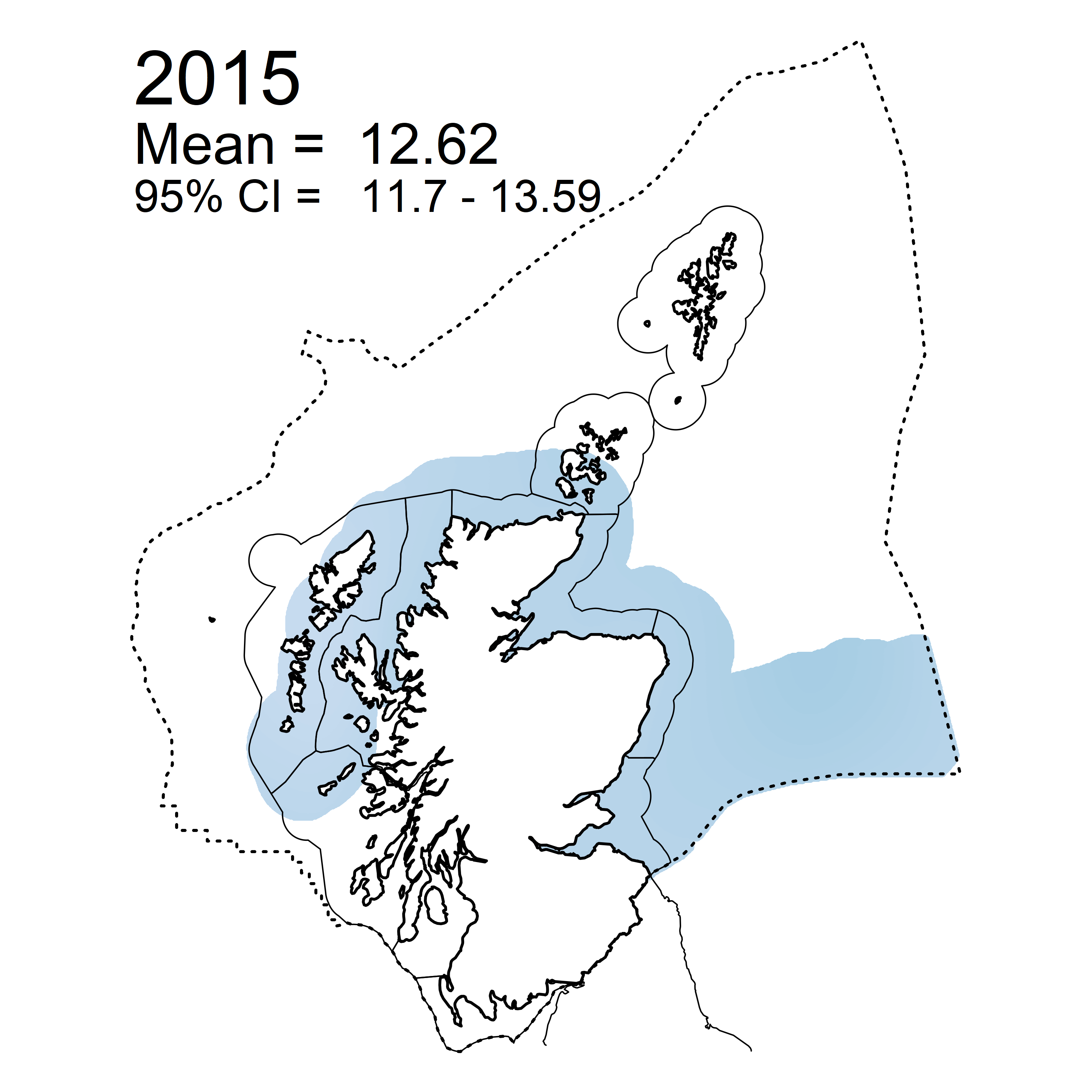
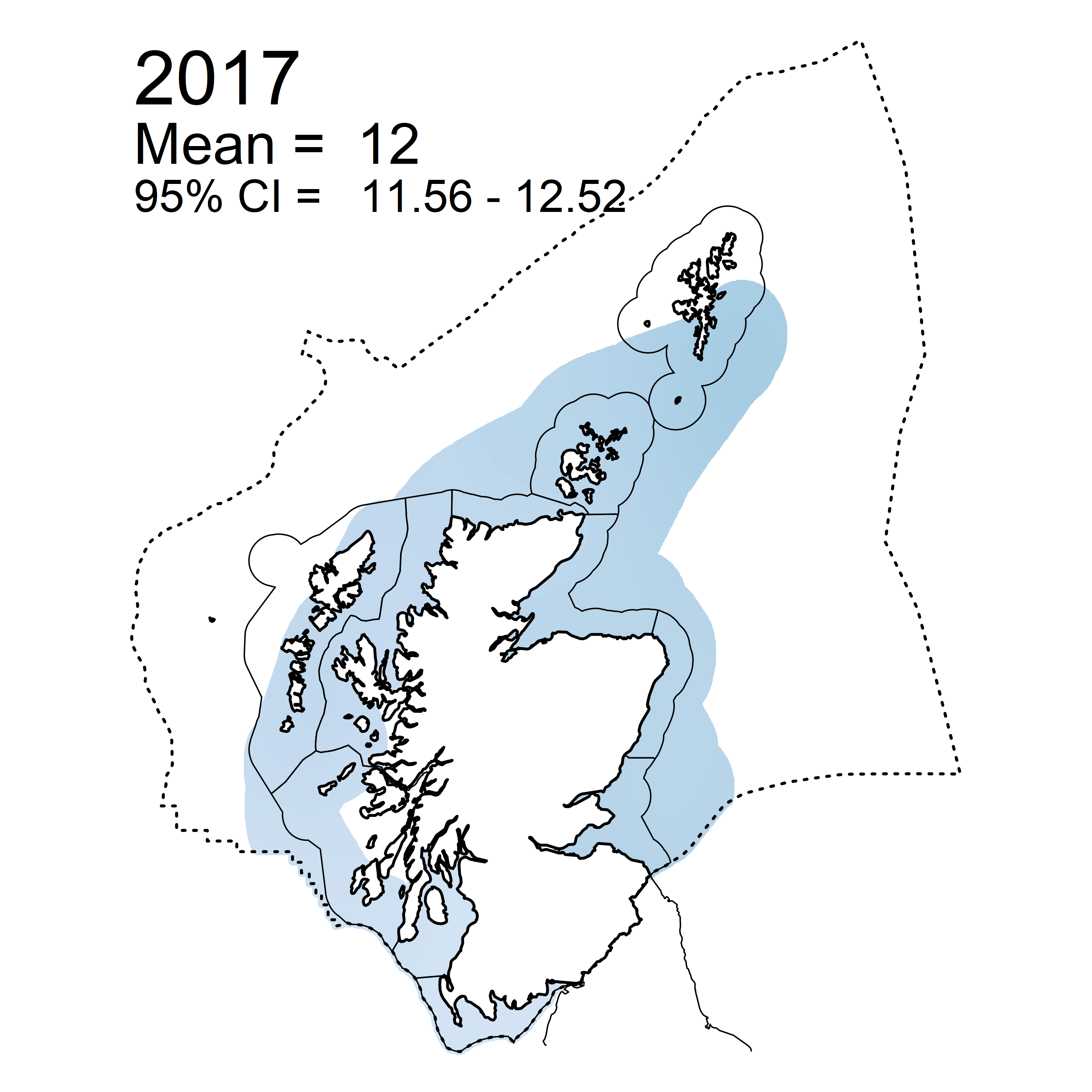
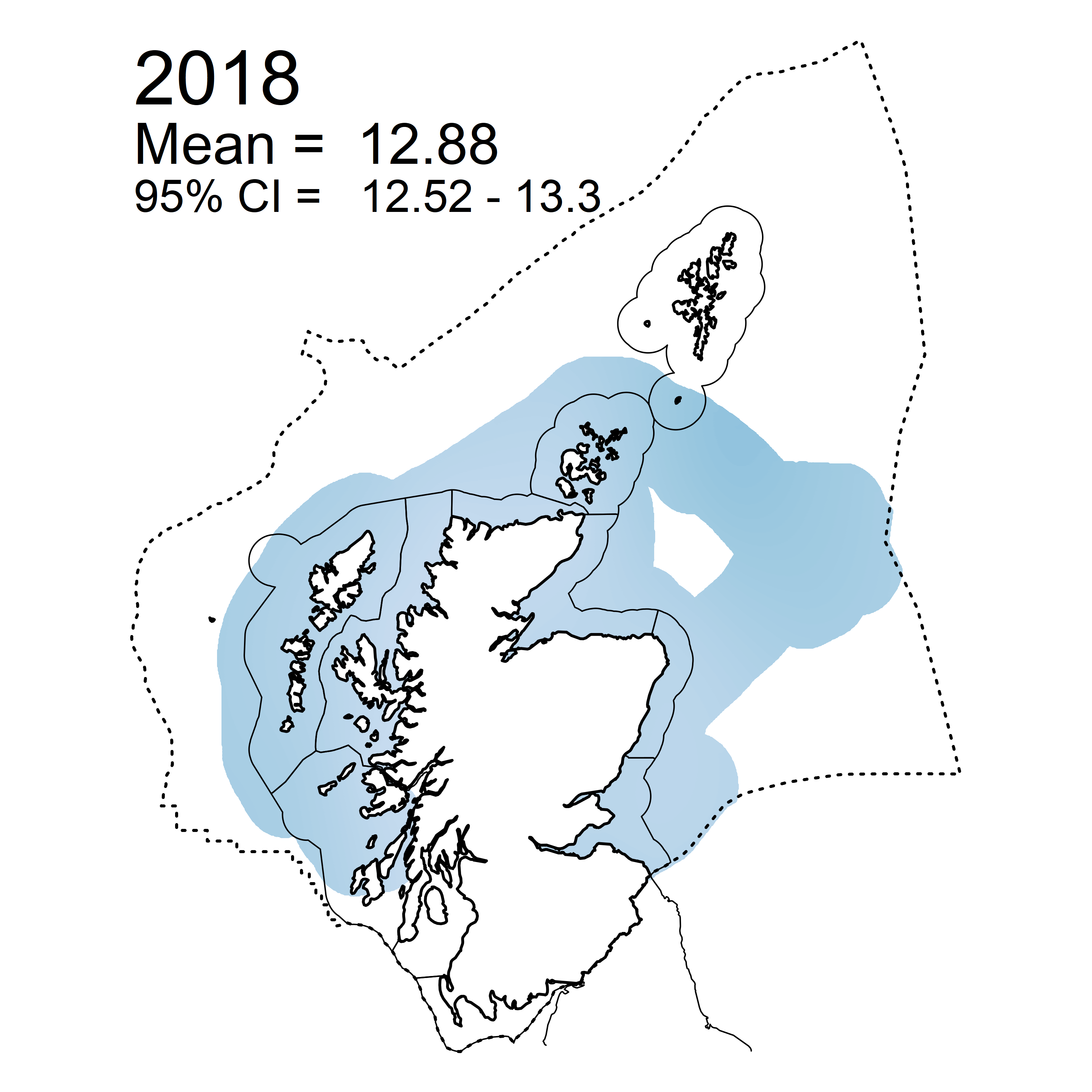
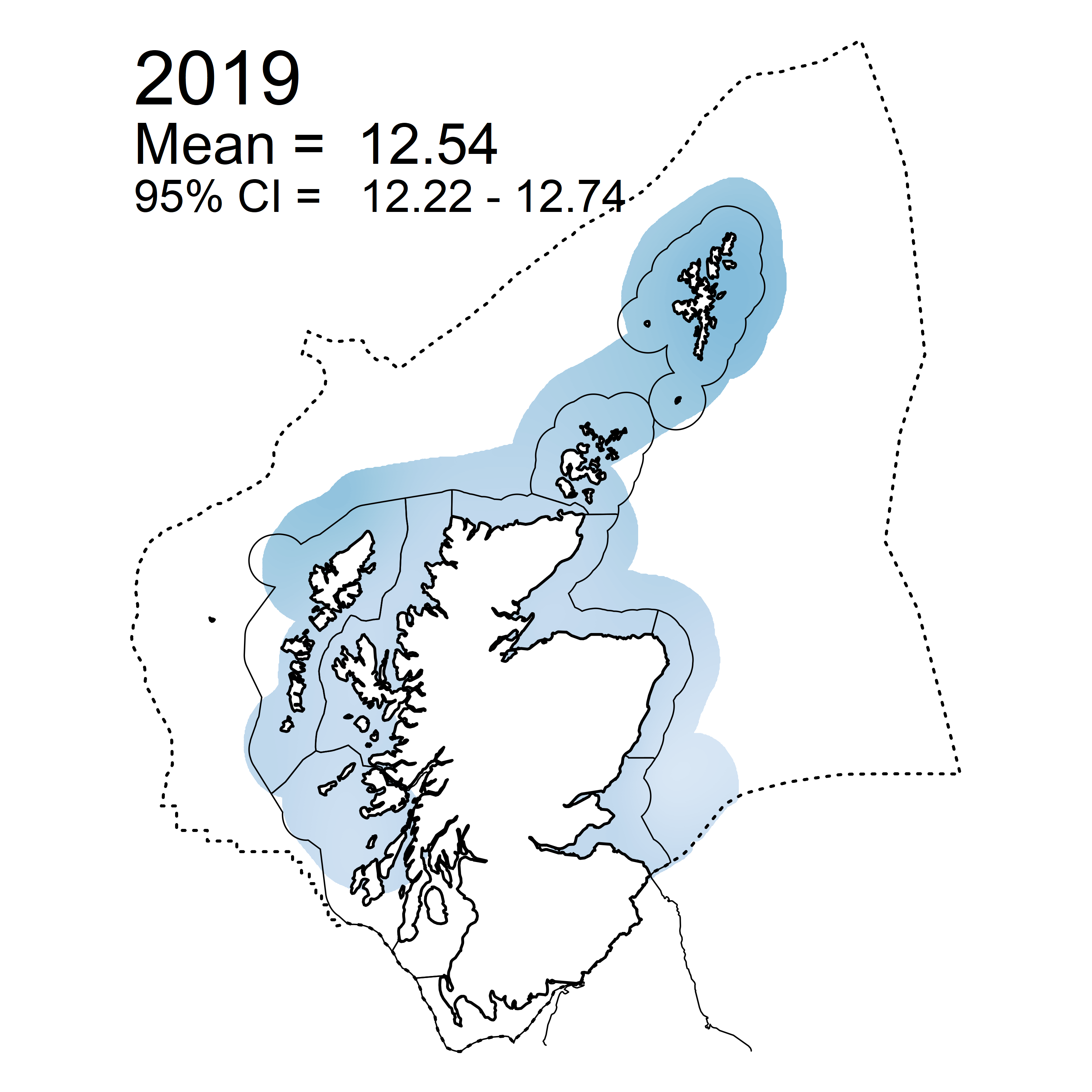
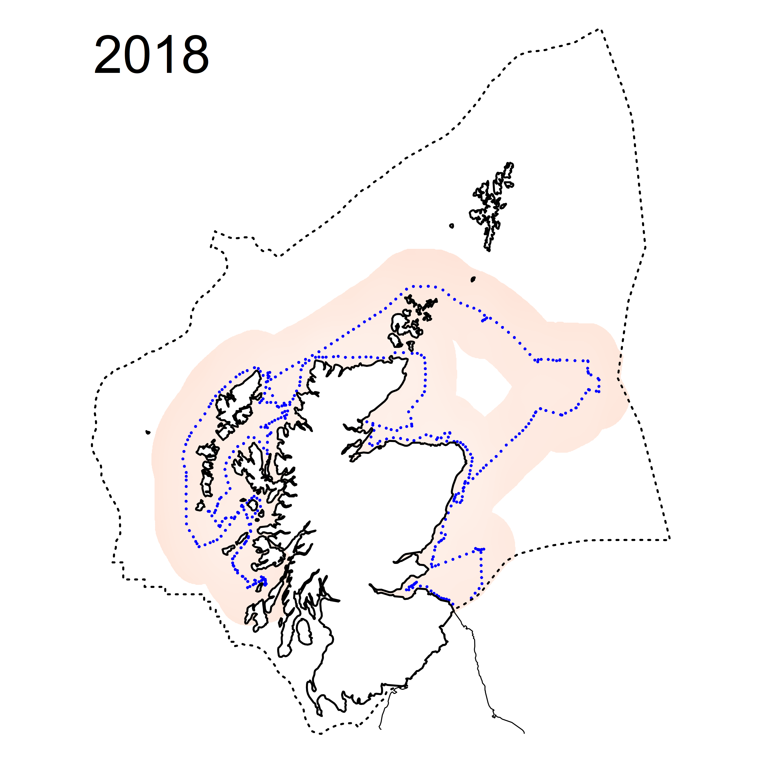
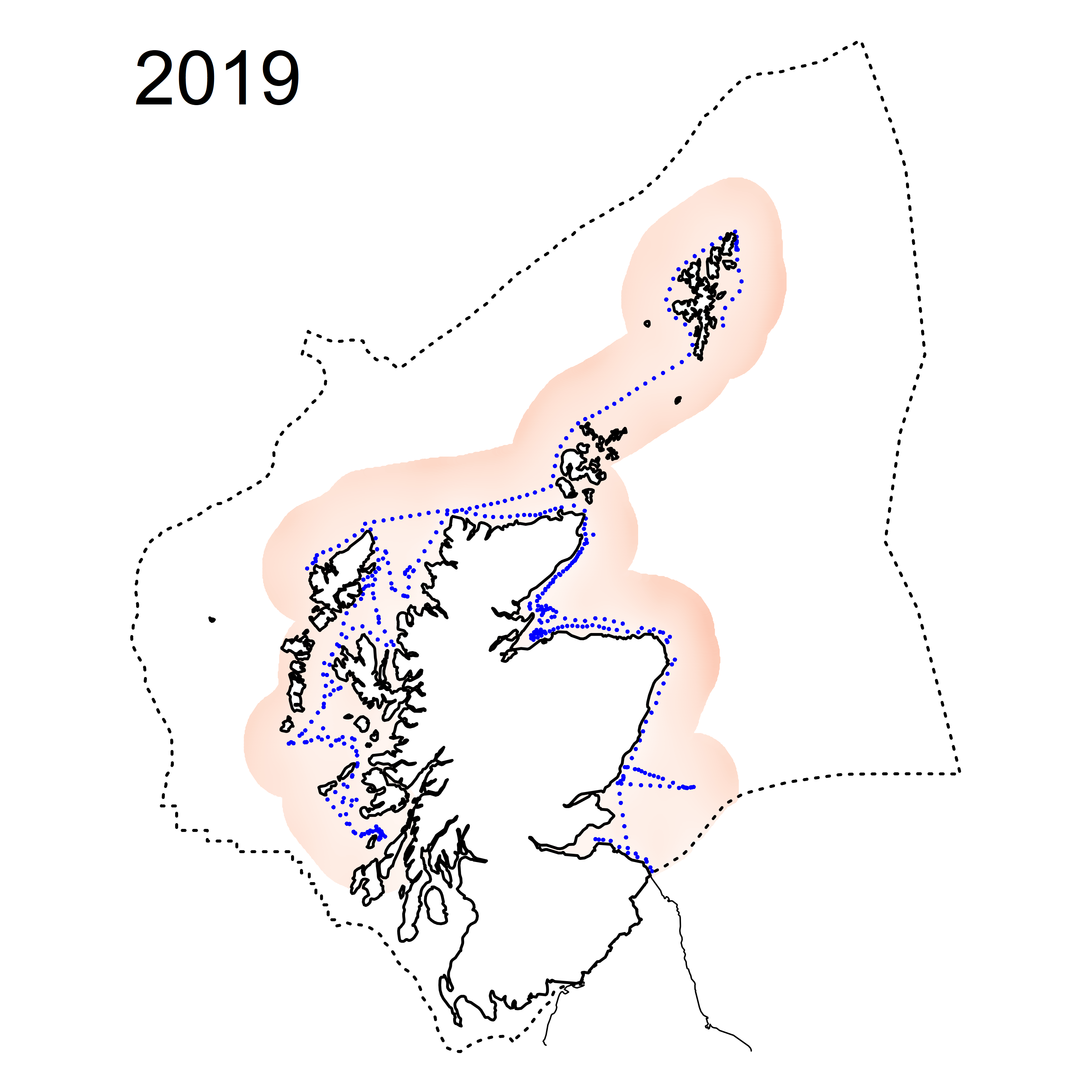
Winter nutrient concentrations have been determined in seawater collected between 2007 and 2019 from coastal and offshore waters. Modelled nutrient concentrations and nutrient ratios have been determined for the eleven SMRs using data from discrete sampling points (Figure 3).

Concentrations were assessed against the OSPAR Ecological Quality Objectives (EcoQOs) for nutrient enrichment in the UK, for dissolved inorganic nitrogen (DIN) (the sum of the concentration of Total Oxidised Nitrogen (TOxN) and ammonia) and the ratio of DIN to DIP. The ammonia contribution to the DIN concentration in offshore water is negligible in Scottish shelf seas and consequently TOxN concentrations can be considered as a proxy for DIN in this assessment.

SMRs encompass both coastal (salinity of 30 - 34.5) and offshore (salinity >34.5) waters. The elevated DIN EcoQOs of 15 µM (offshore waters) and 18 µM (coastal waters) and the coastal background concentration (12 µM), were not exceeded in any SMR. Most regions also had concentrations below the offshore background concentration (10 µM) (Figure 3). TOxN concentrations were stable in all SMRs over the assessment period (Figure 3).

This is in contrast to the nutrient input assessment which showed significant increases for total nitrogen in Orkney and the Outer Hebrides, which indicates this may be a consequence of localised point sources such as aquaculture, with nitrogen not readily available in the wider marine region or dispersion/ dilution in the region.

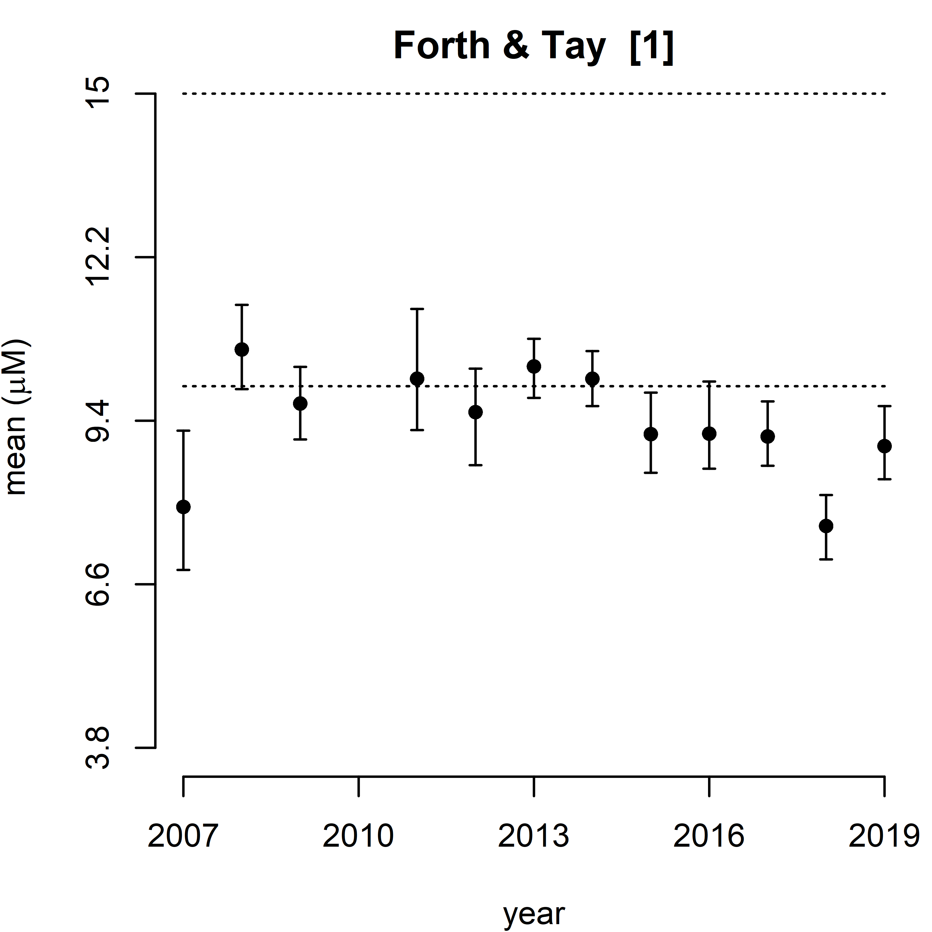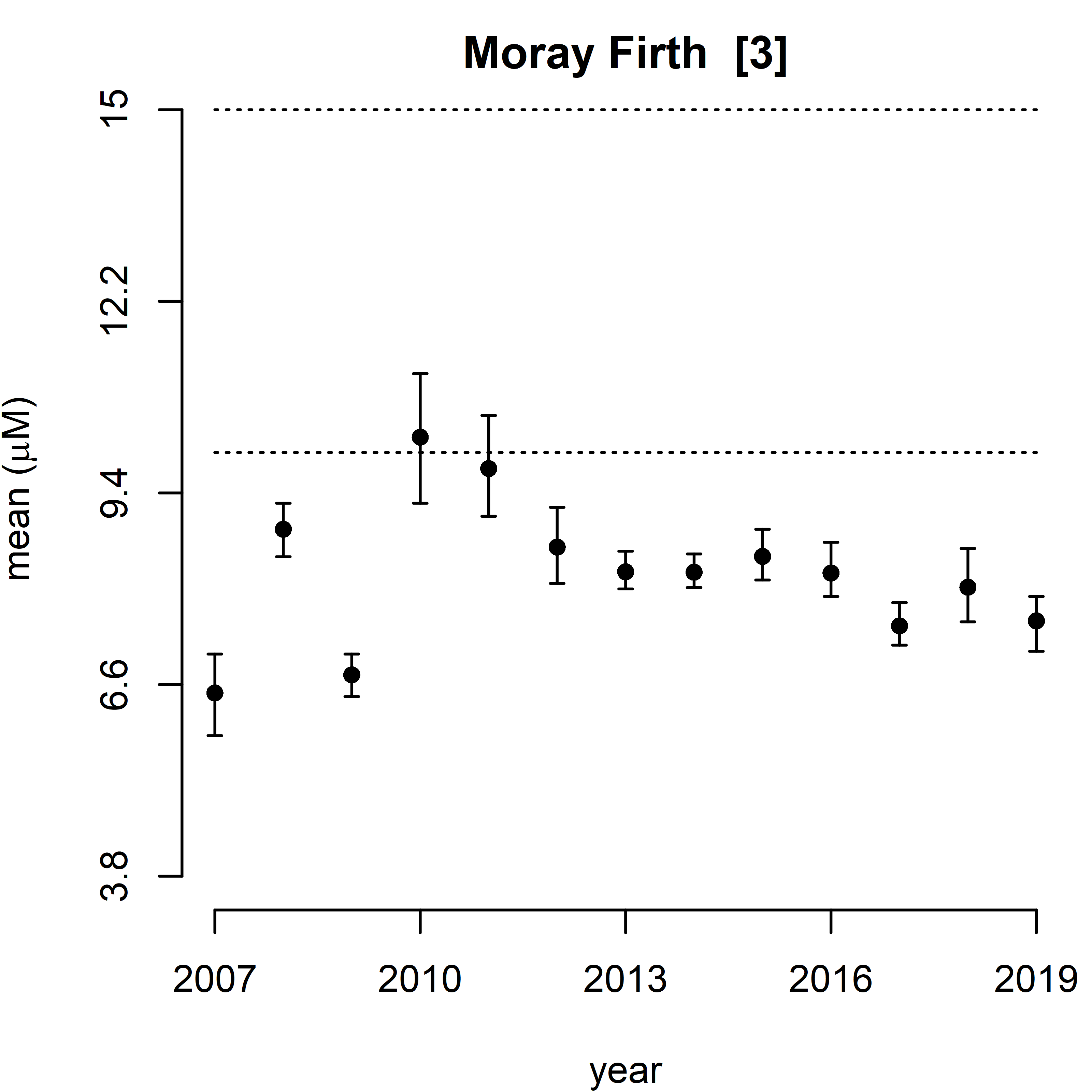
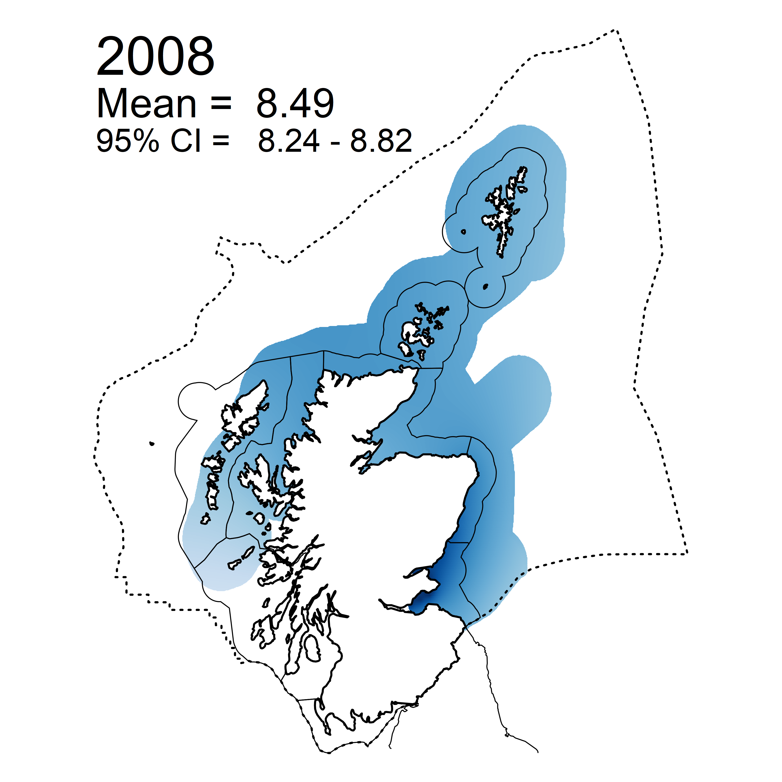
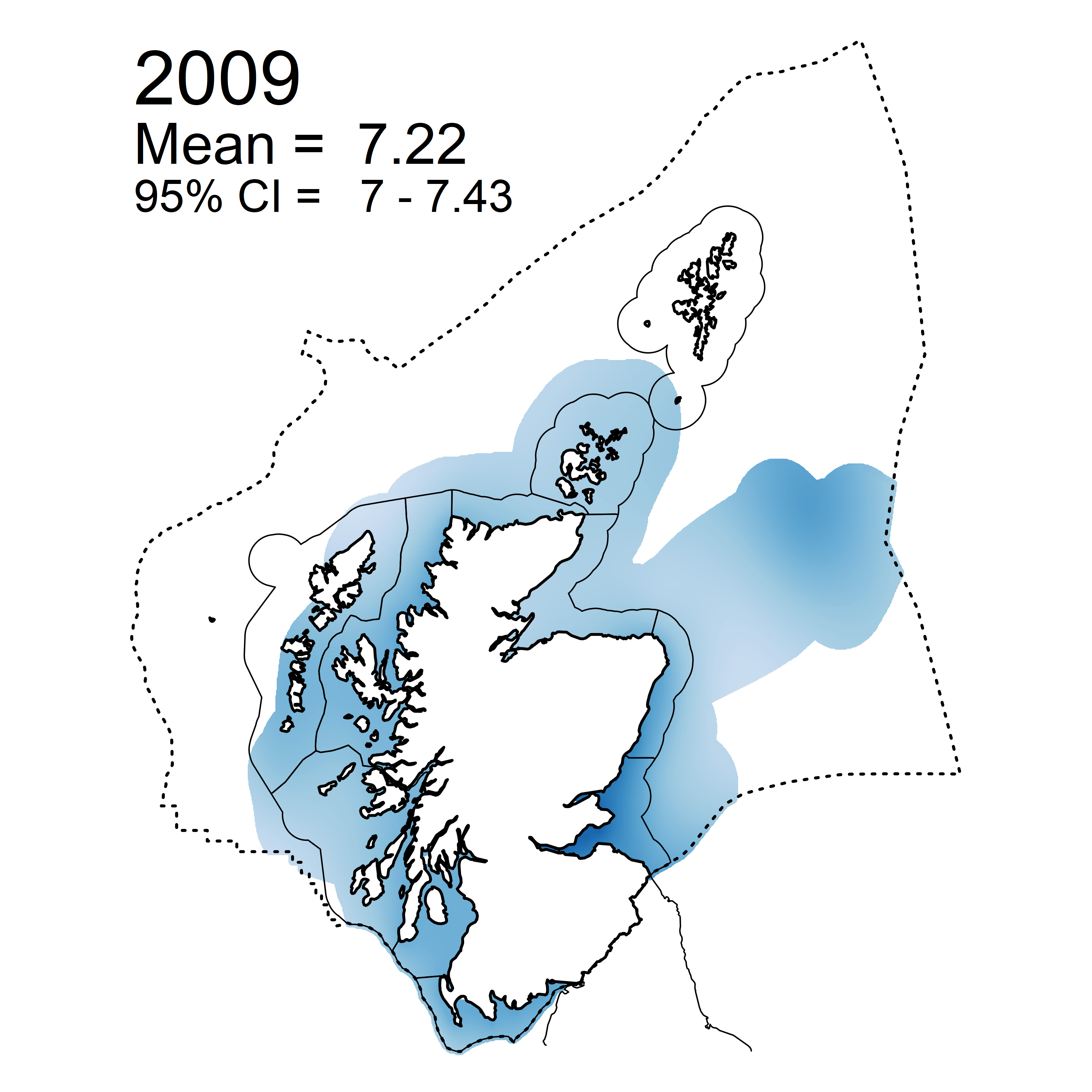
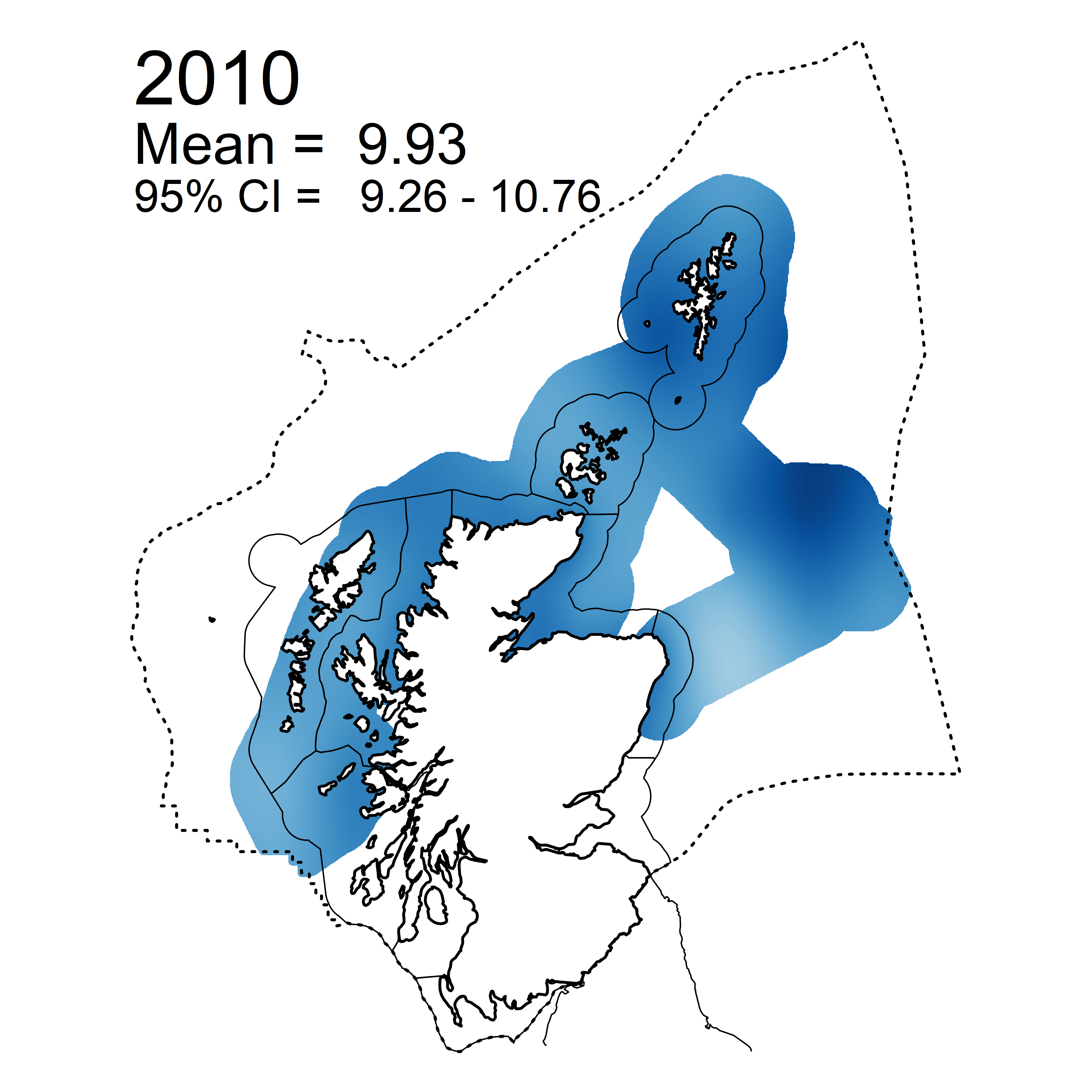
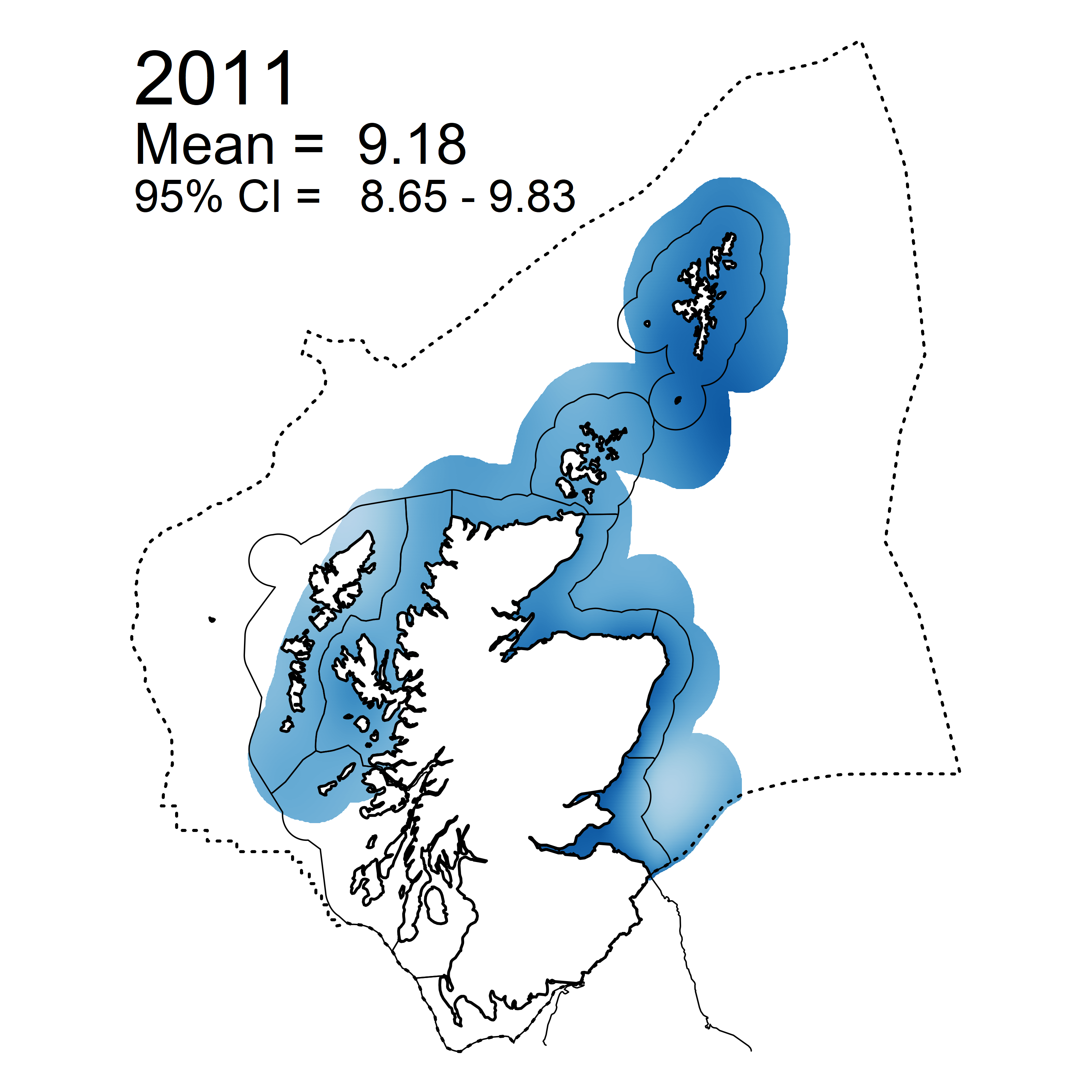
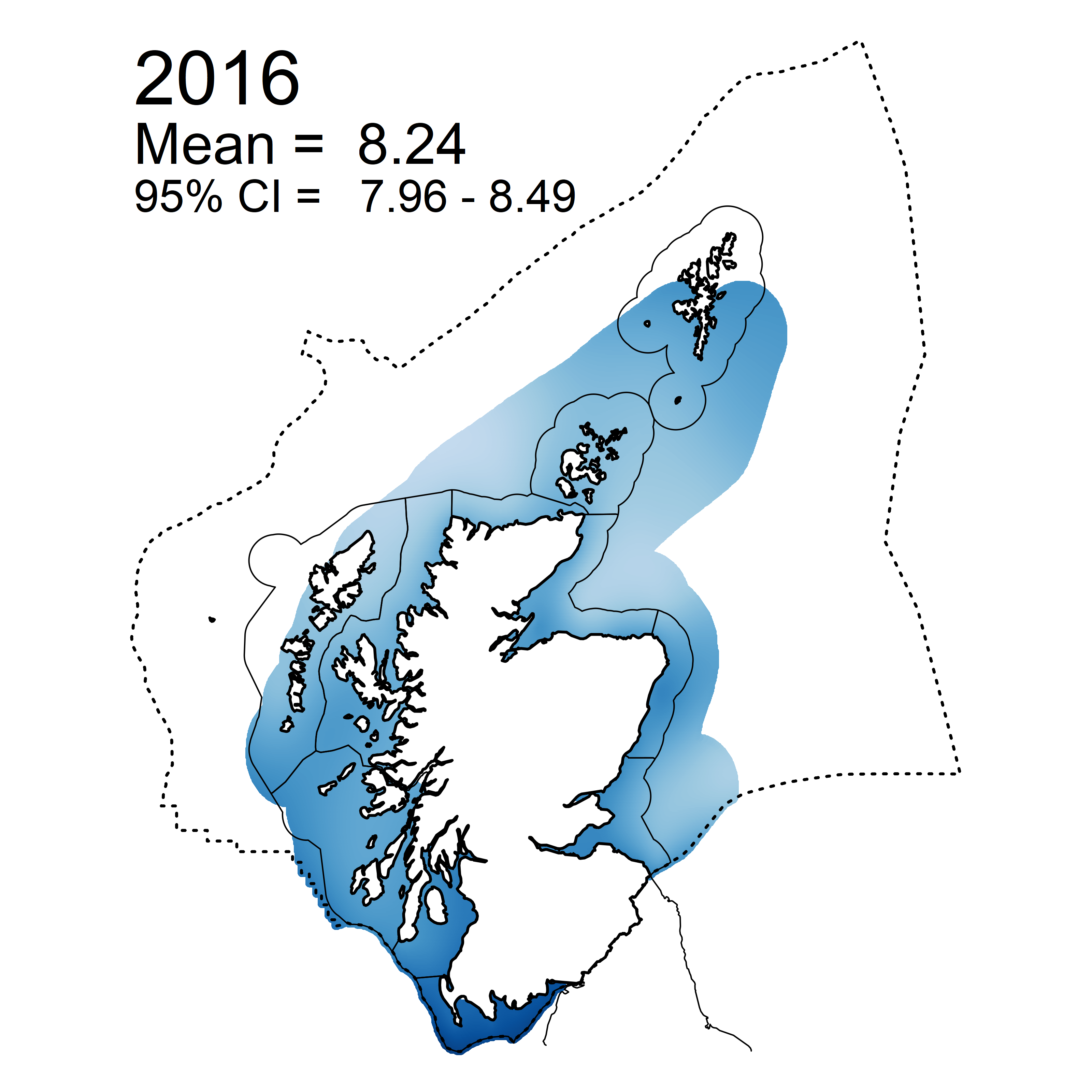
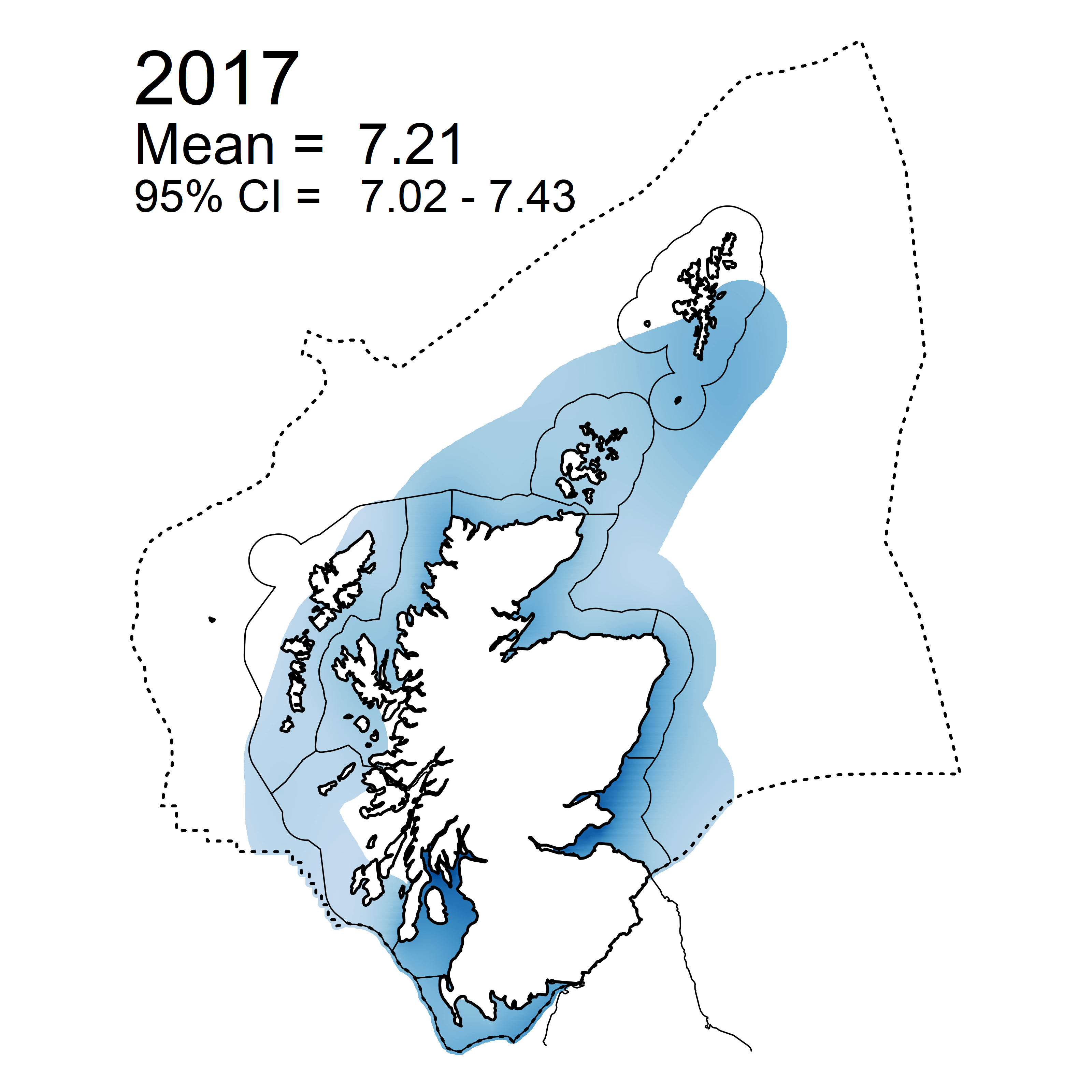
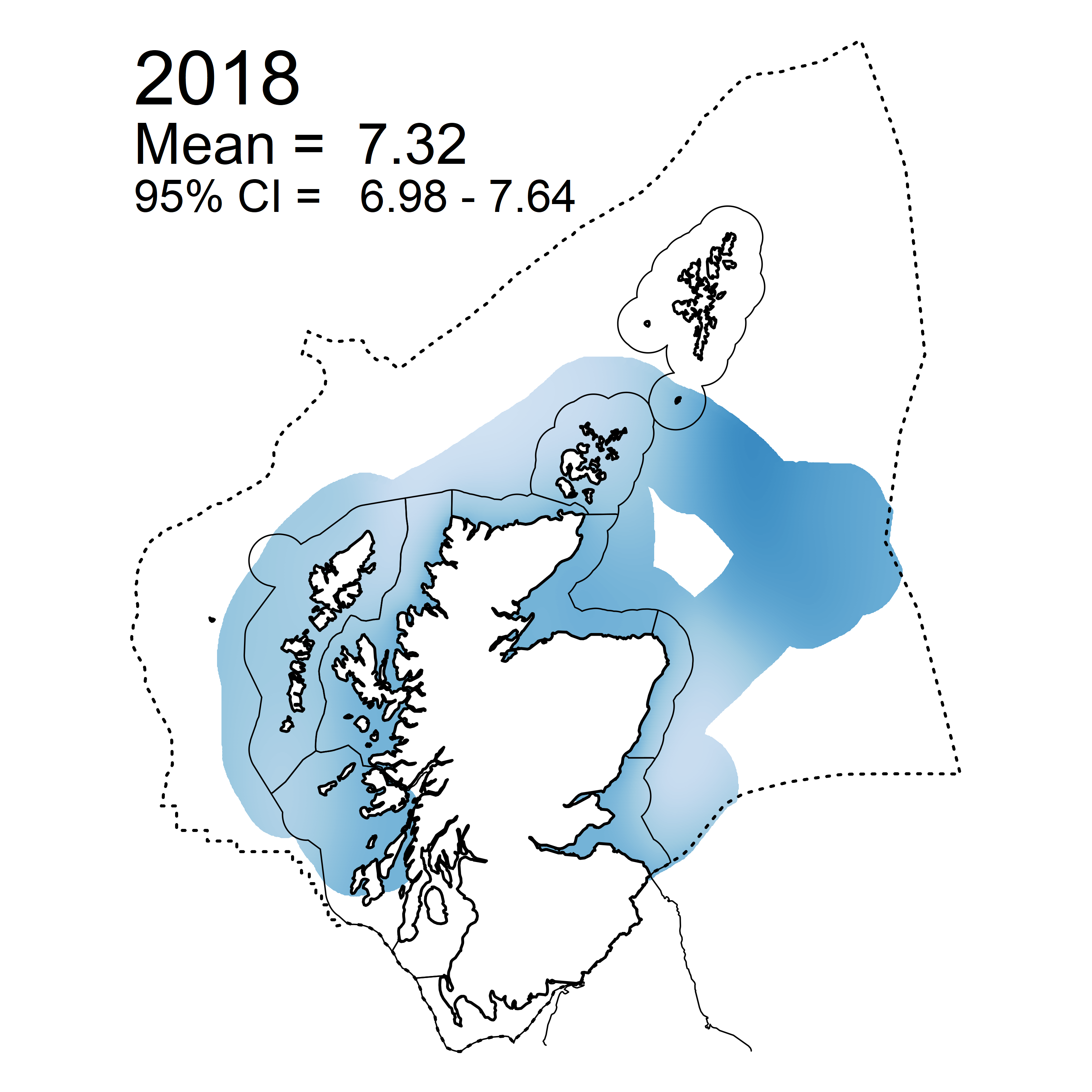
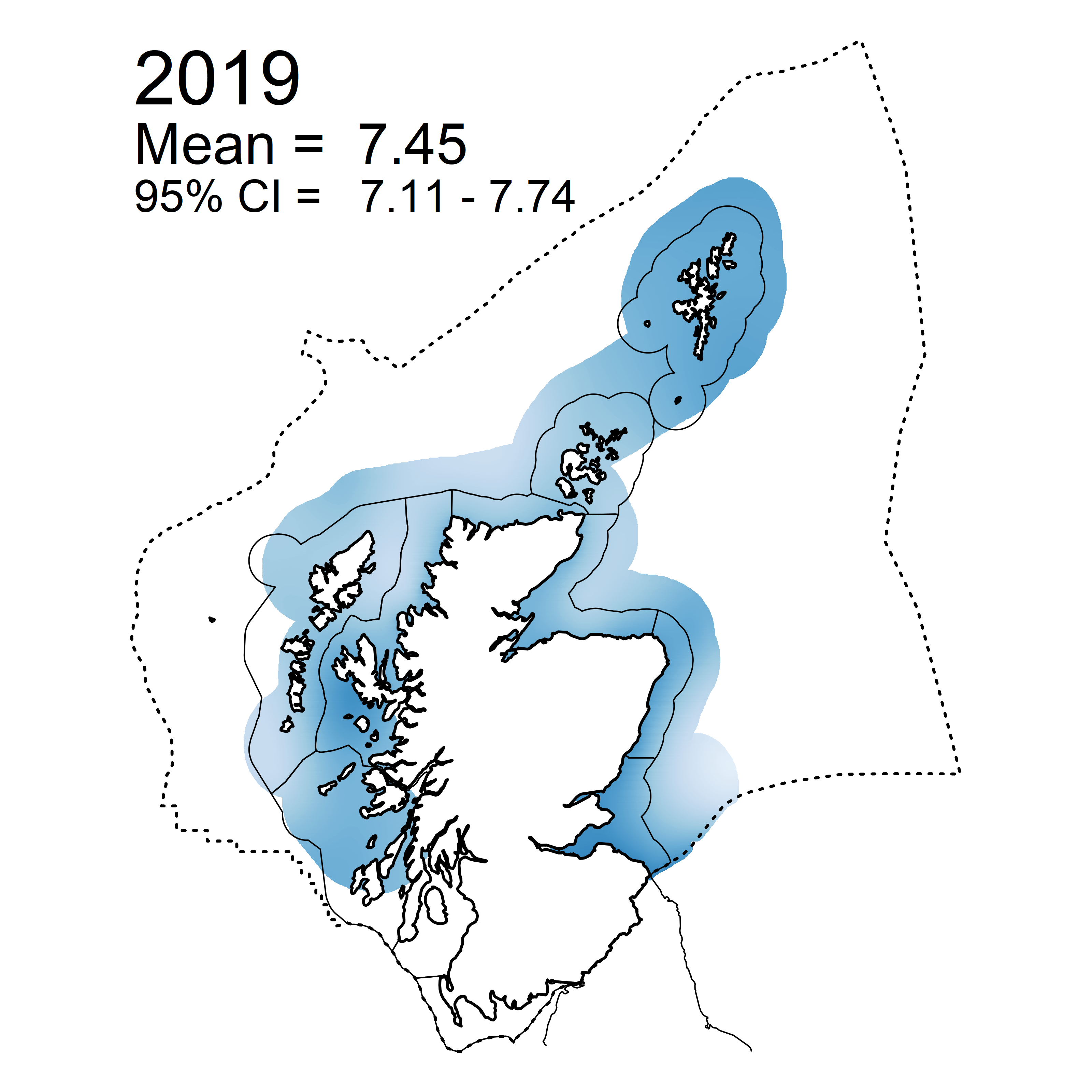
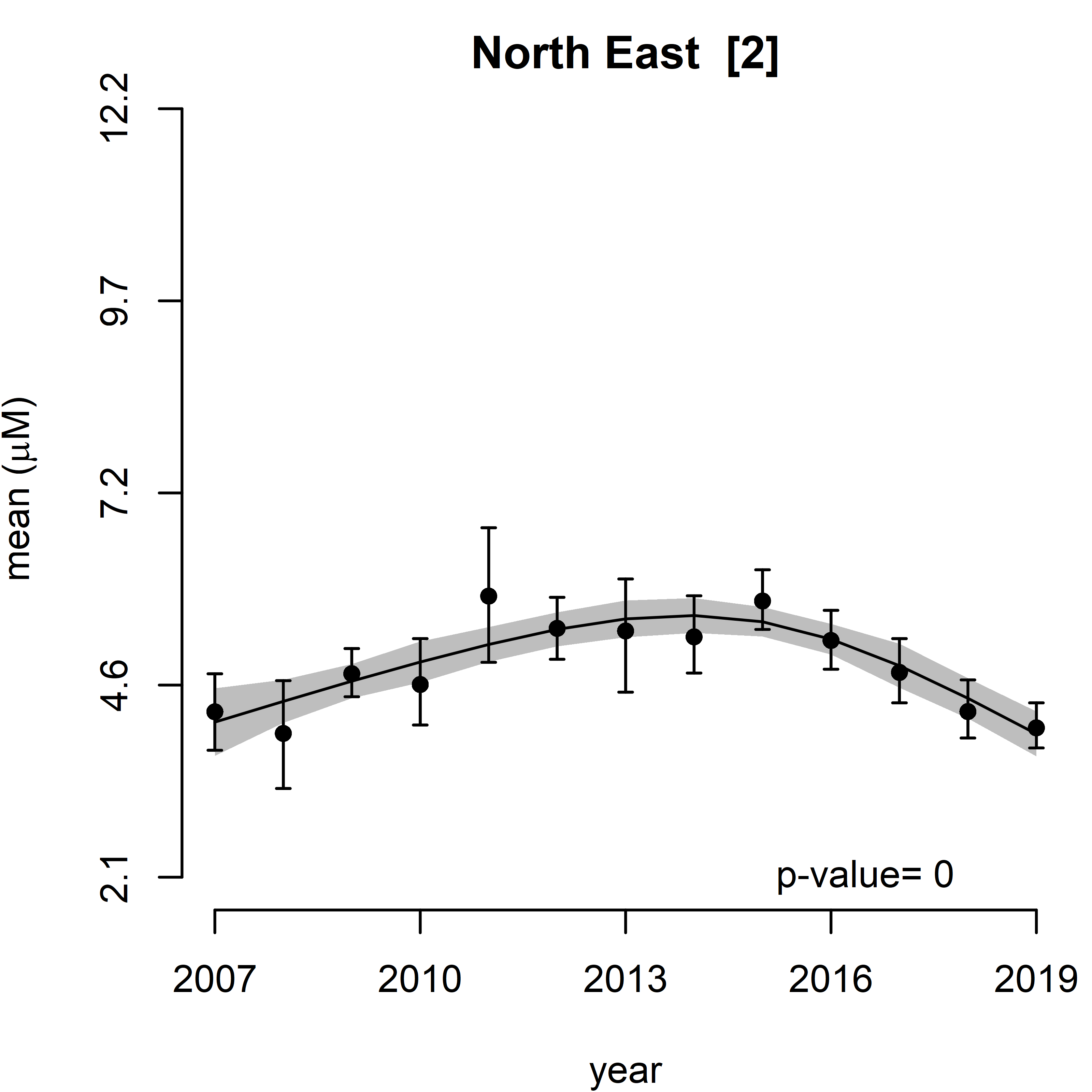
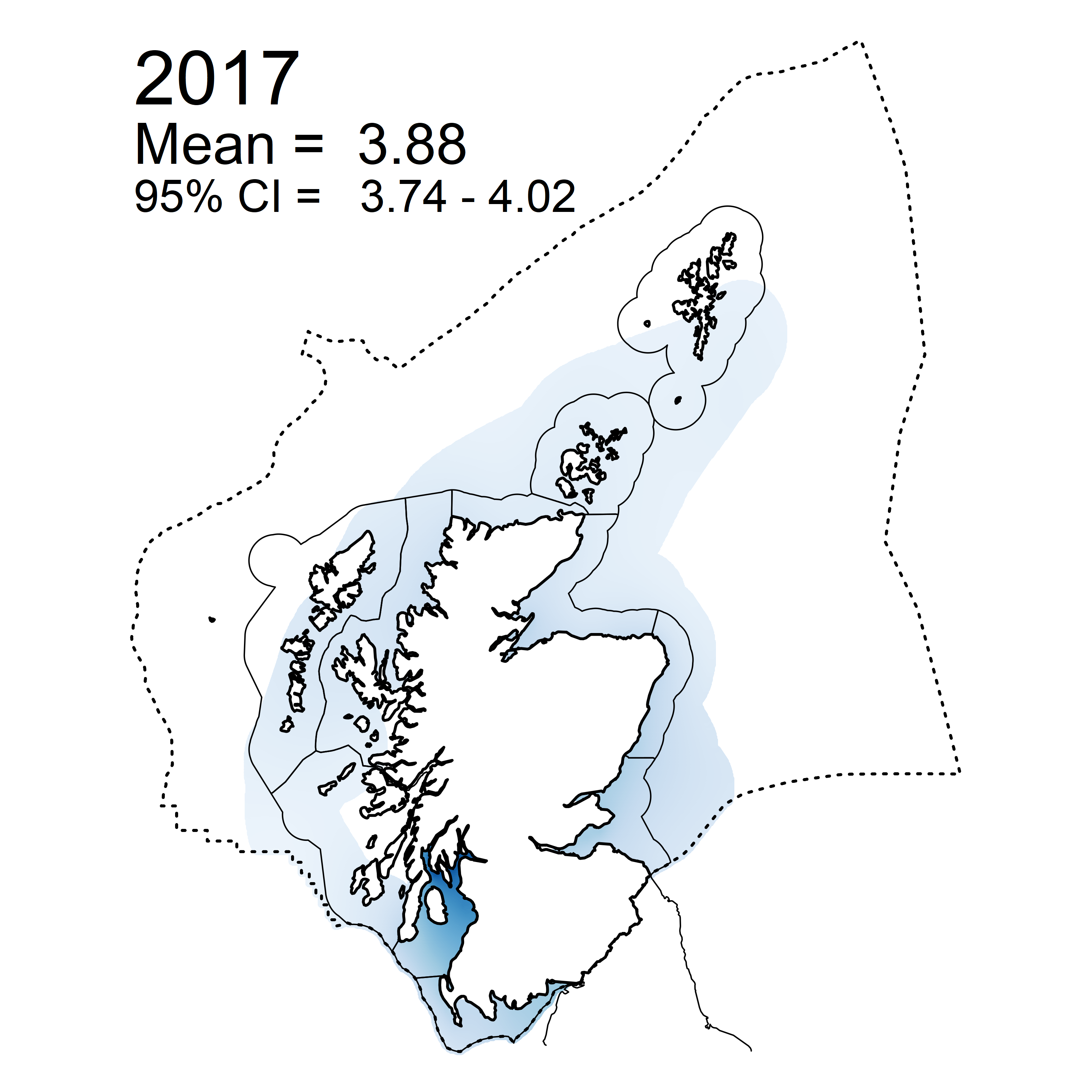
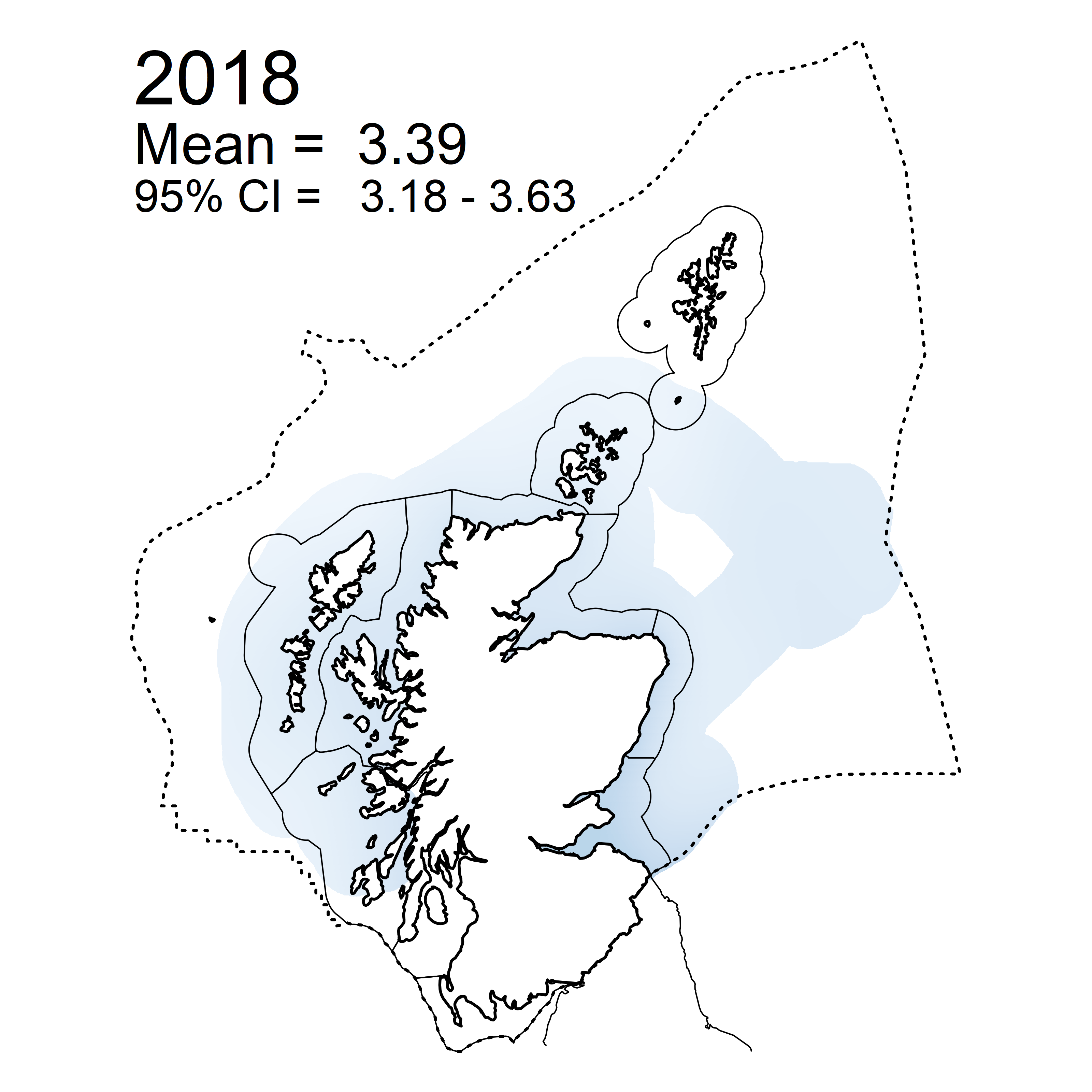
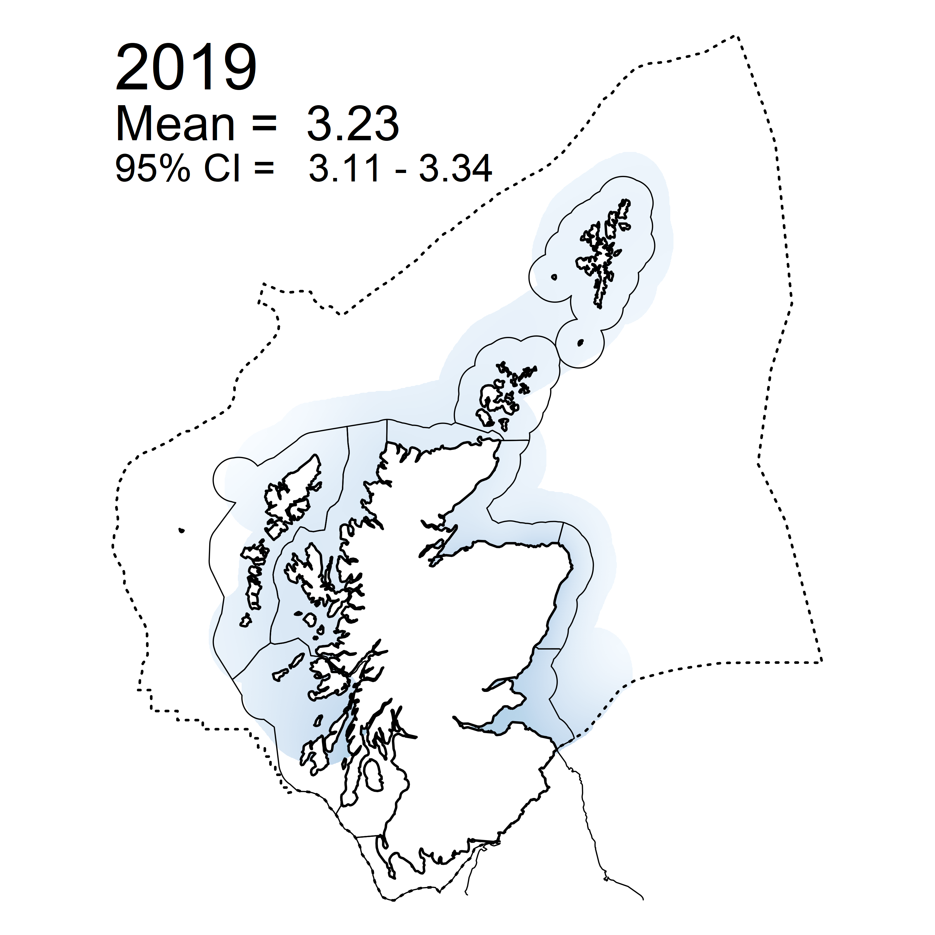
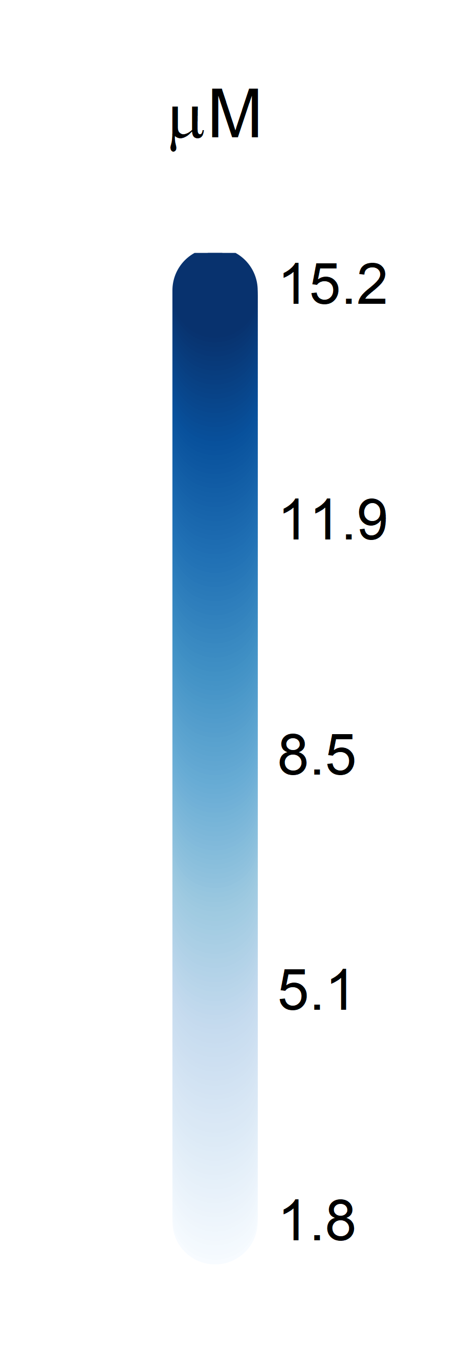
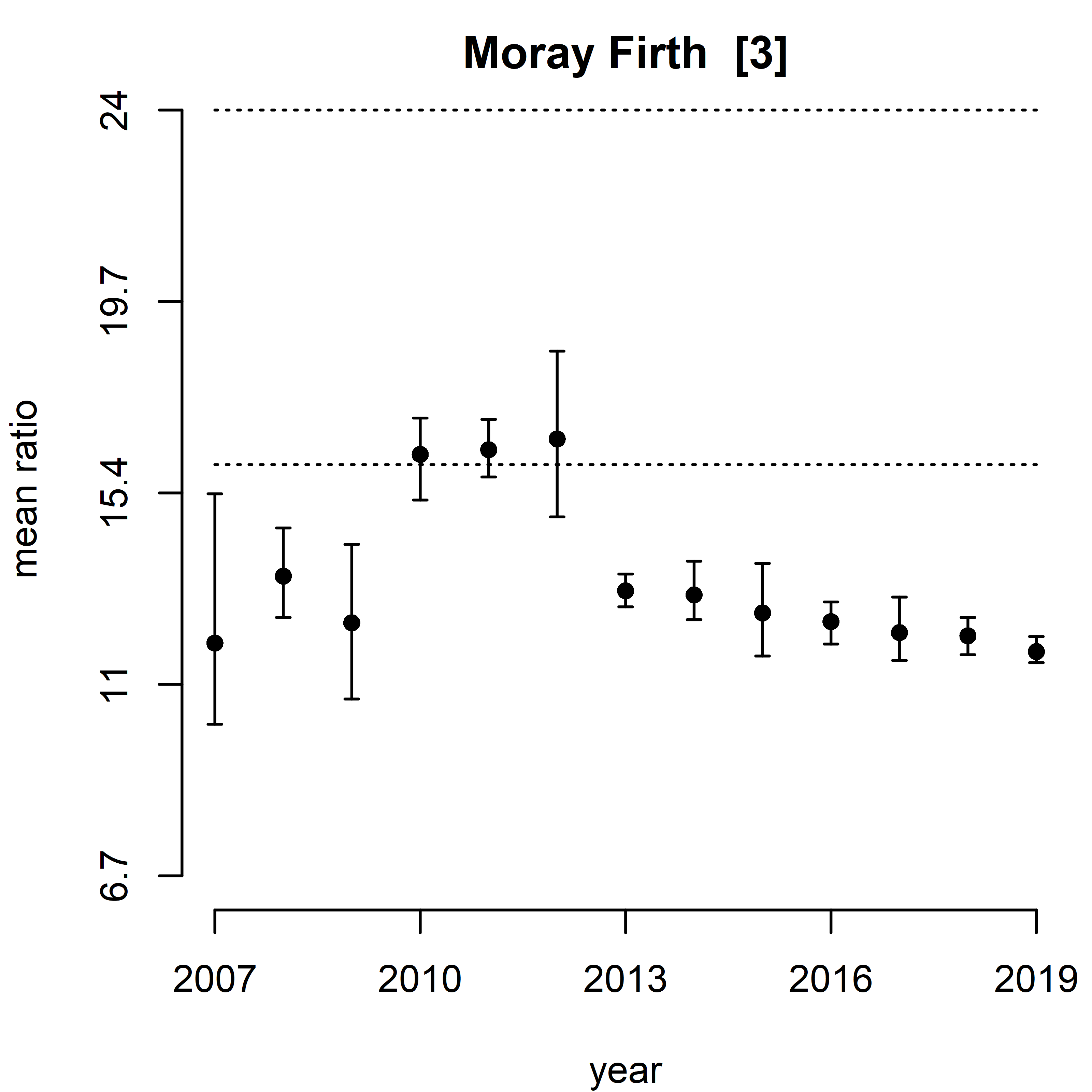
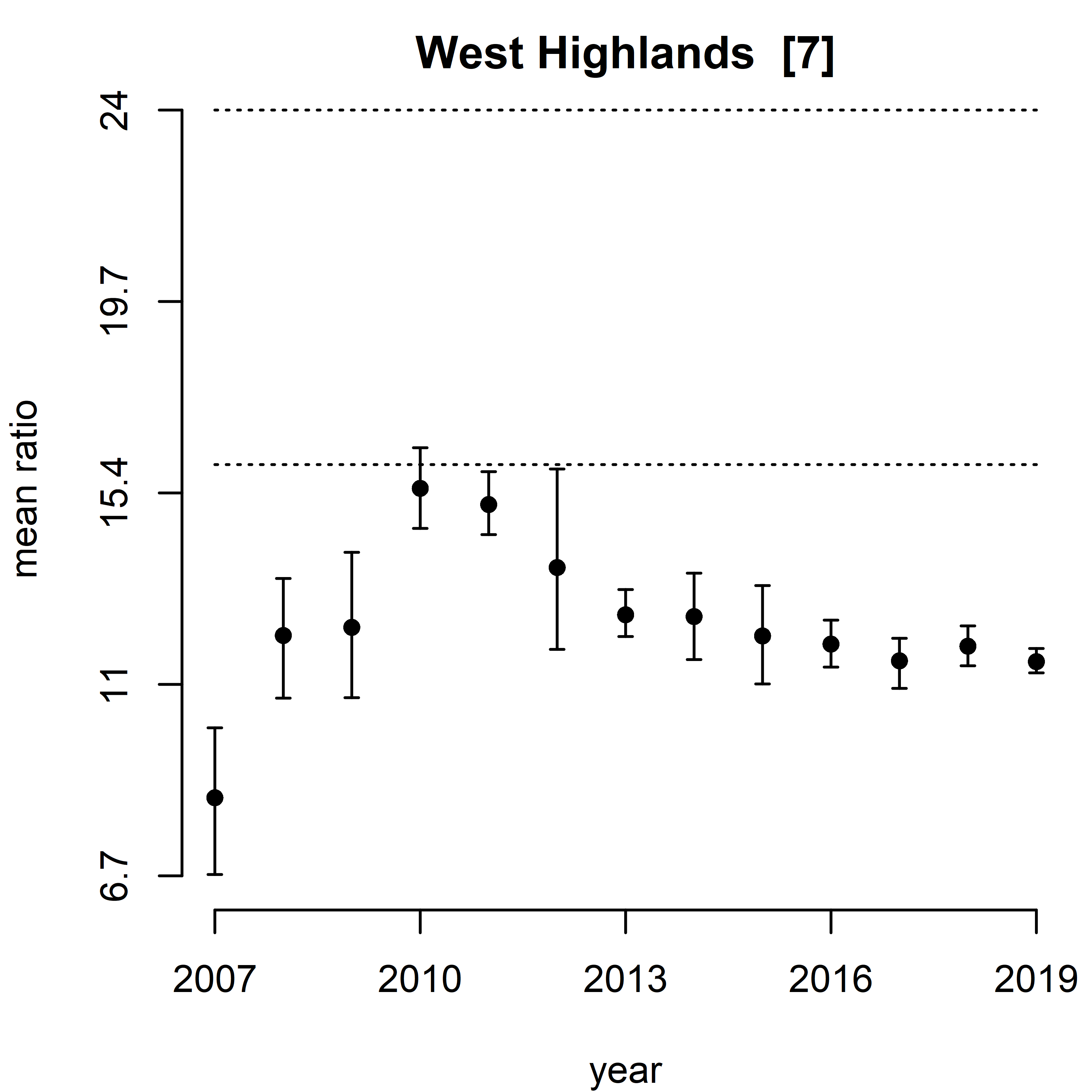
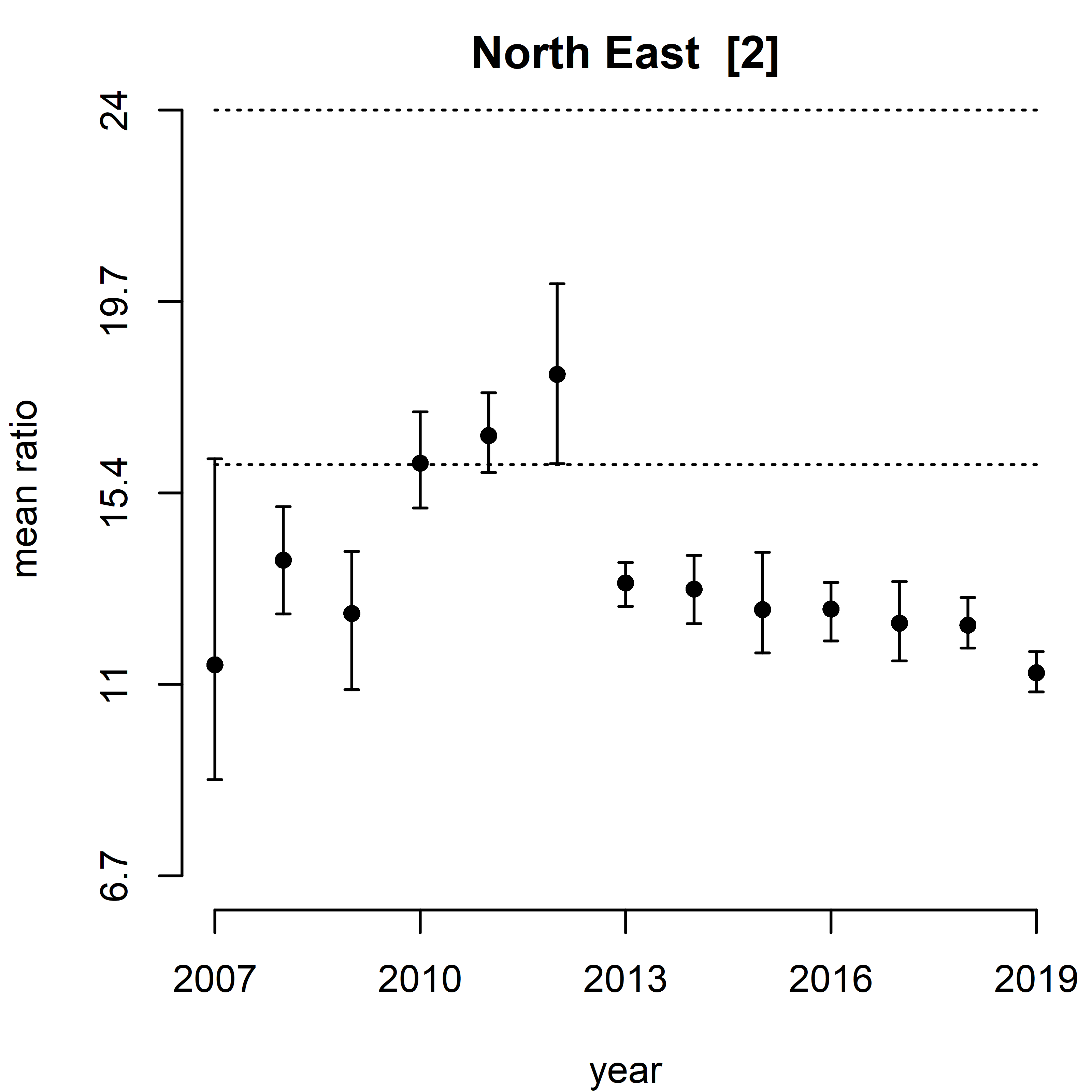
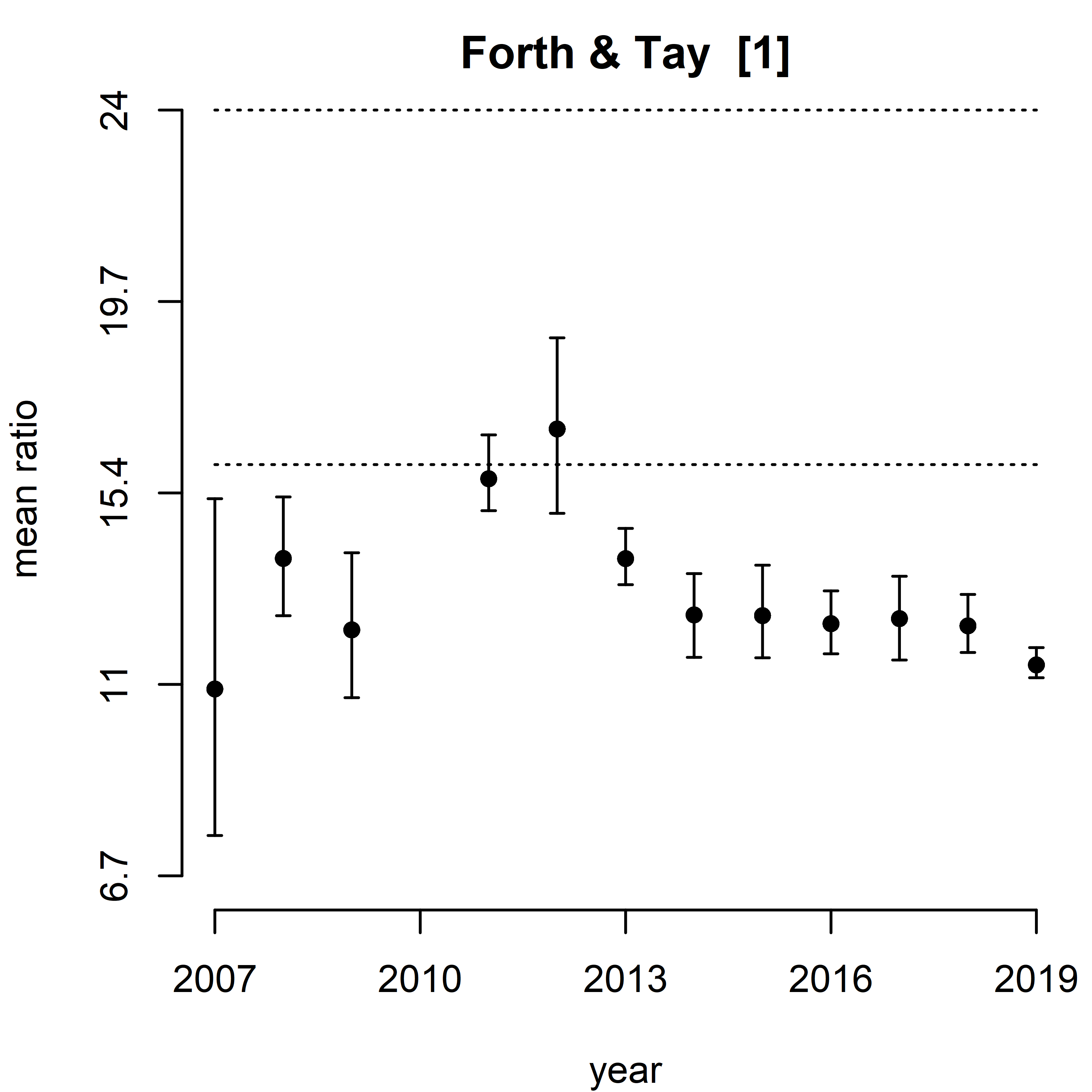
Figure 3: Summary plot of modelled salinity normalised total oxidised nitrogen (TOxN) for winters 2017-2019 (map) for Scottish waters and mean predicted trends over the time series (2007-2019) (graphs). The hashed lines, in the trend assessment, correspond to offshore background (10 µM) and assessment levels (15 µM) for winter offshore DIN concentrations. The Scottish Marine Regions (SMR) are identified as 1-11 corresponding to; SMR 1 Forth and Tay, SMR 2 North East, SMR 3 Moray Firth, SMR 4 Orkney Islands, SMR 5 Shetland Isles, SMR 6 North Coast, SMR 7 West Highlands, SMR 8 Outer Hebrides, SMR 9 Argyll, SMR 10 Clyde & SMR 11 Solway. Mean values were only estimated for a SMR when the predicted values covered at least 80% of the relevant area.

MSS data were used in the assessment. The laboratory complies with ISO 17025 and is accredited by the UK accreditation service (UKAS) for nutrient analyses. On-going competency is demonstrated through participating in the QUASIMEME proficiency testing scheme. Therefore, there is high confidence in the quality of the data used in this assessment. The data have been collected over many years using established sampling methodologies. In addition, established and internationally recognised protocols for monitoring and assessment are used, therefore there is also high confidence in the methods. The assessment methodology has been developed and improved since Scotland’s Marine Atlas (Baxter et al., 2011), with an assessment of the eleven Scottish Marine Regions being undertaken and presented here rather than on the individual station presented in the Atlas.

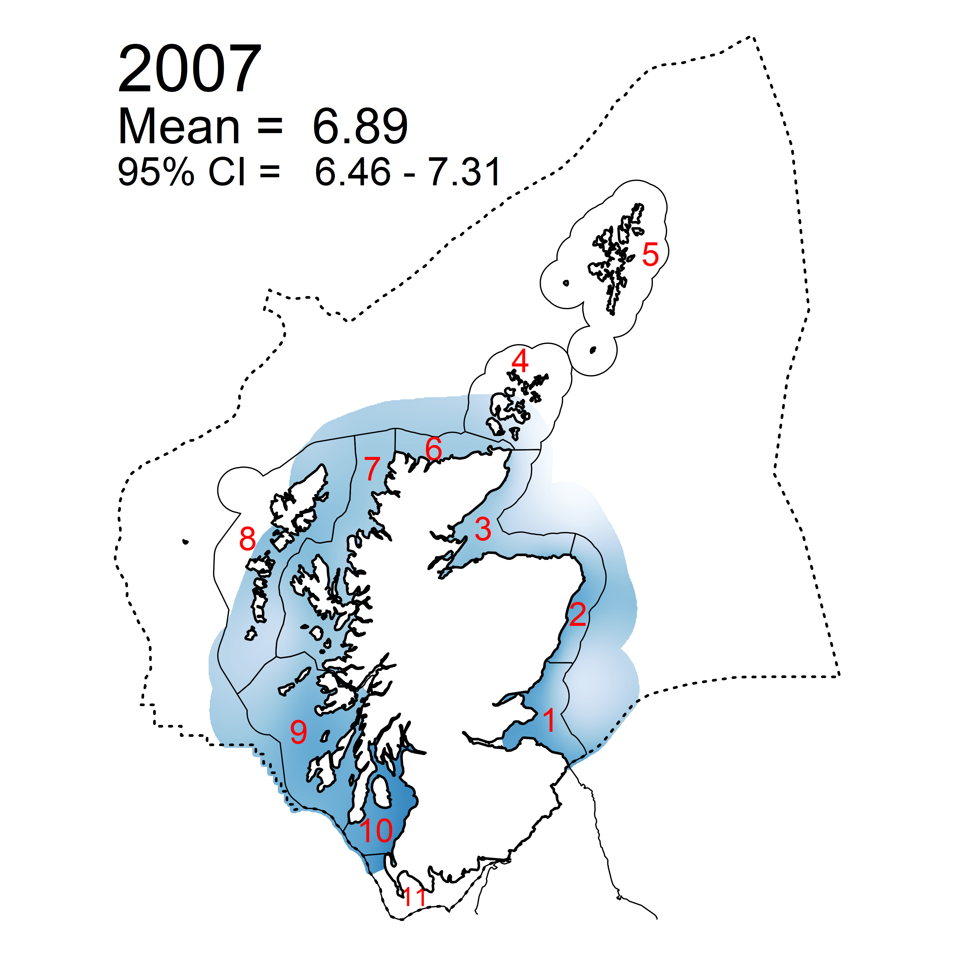
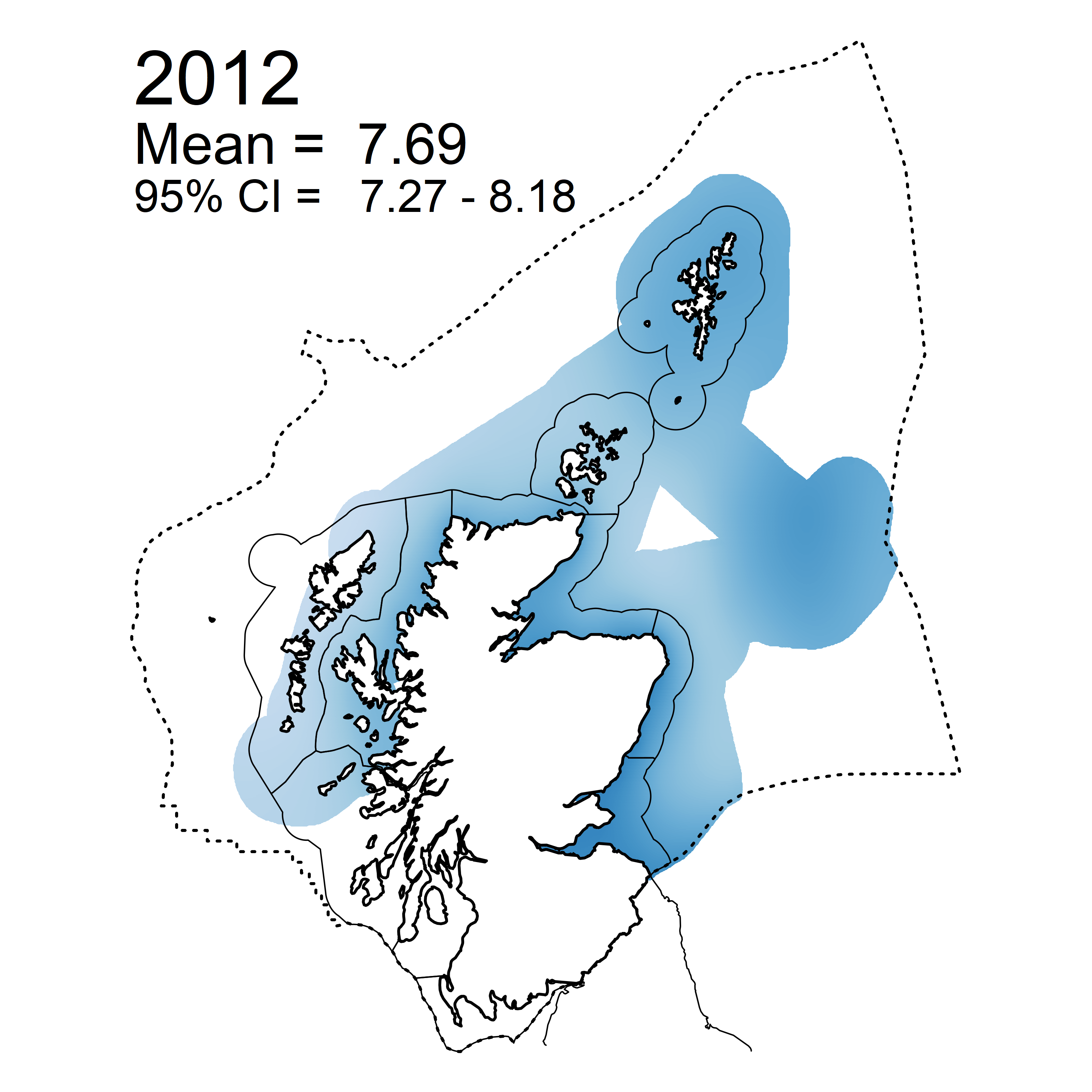
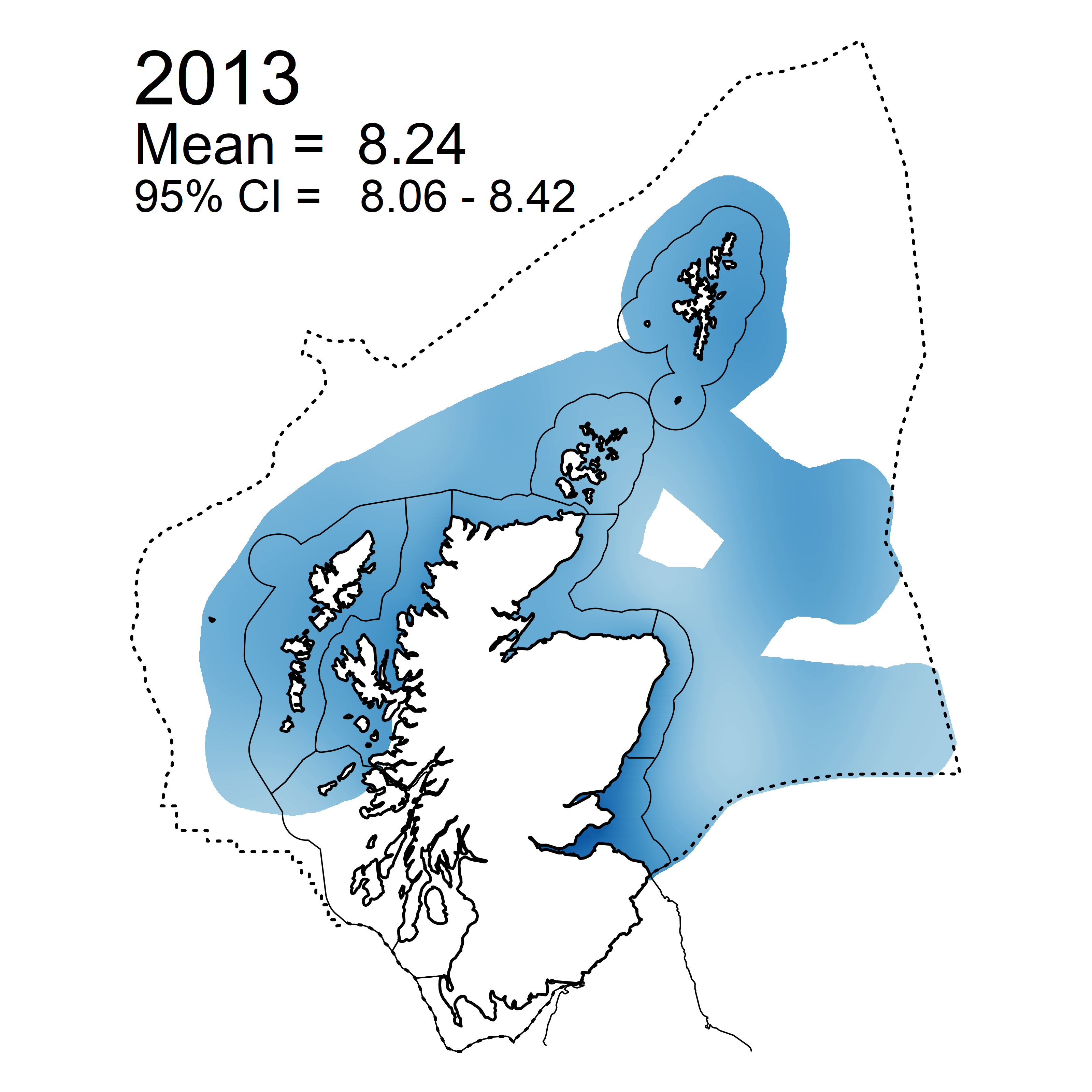
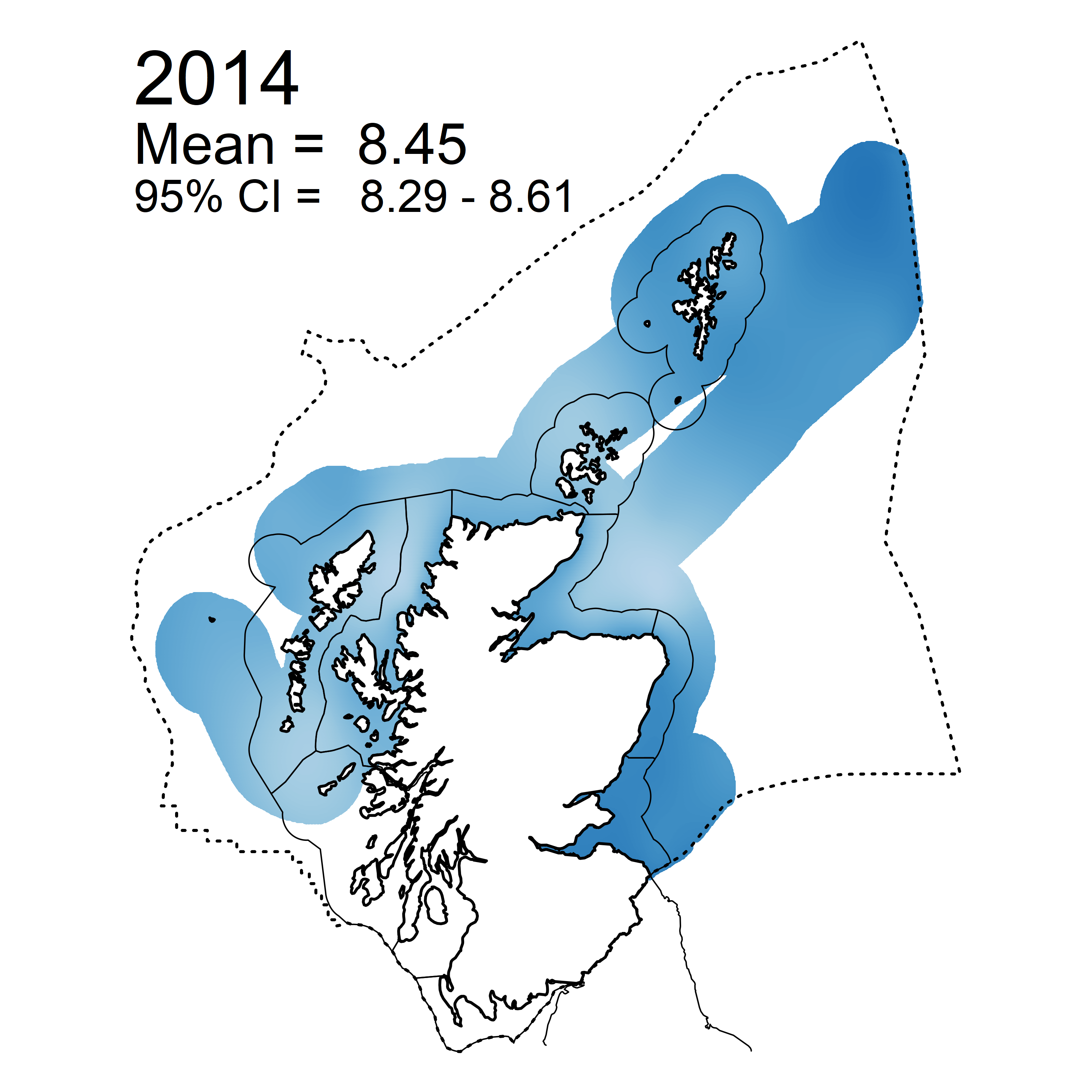
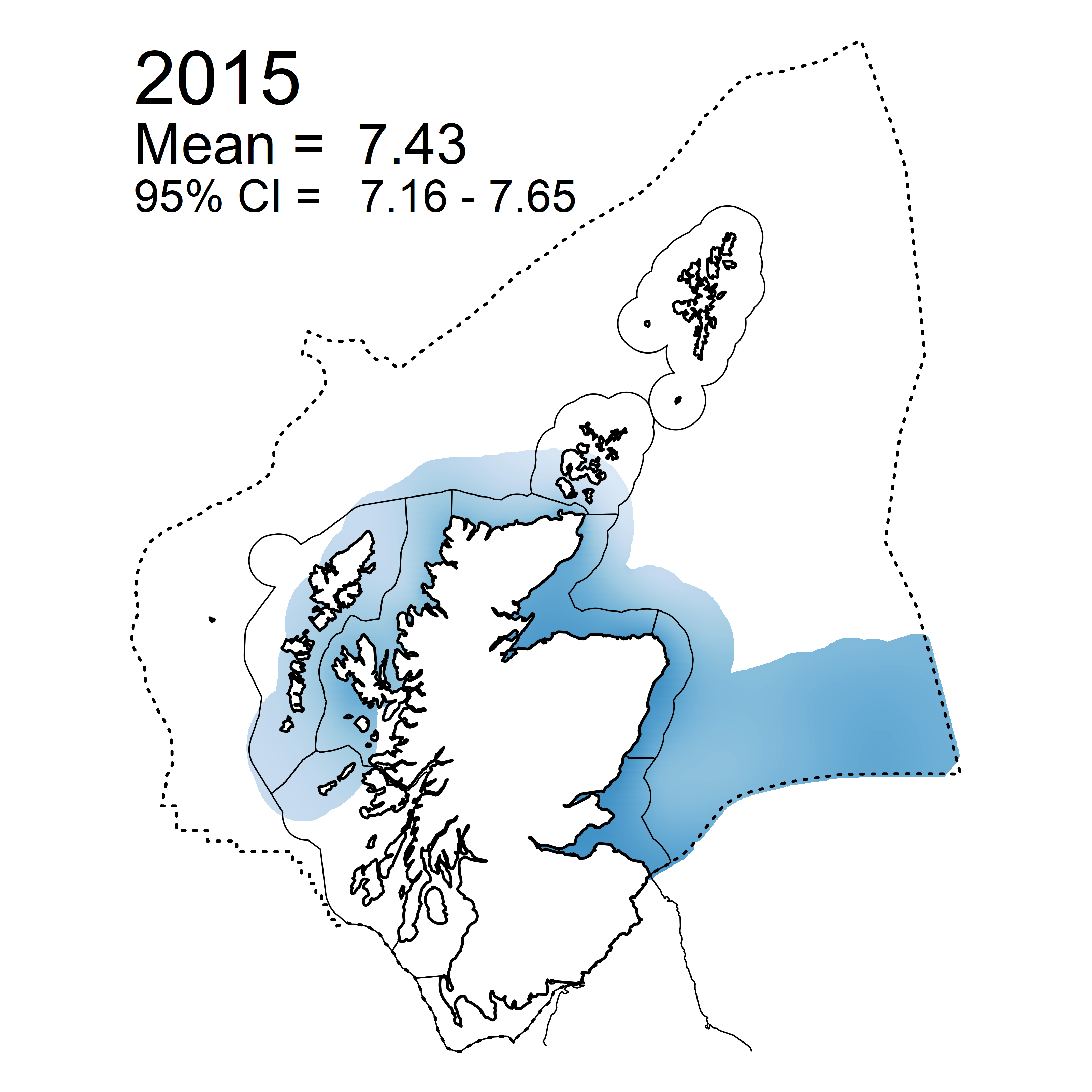
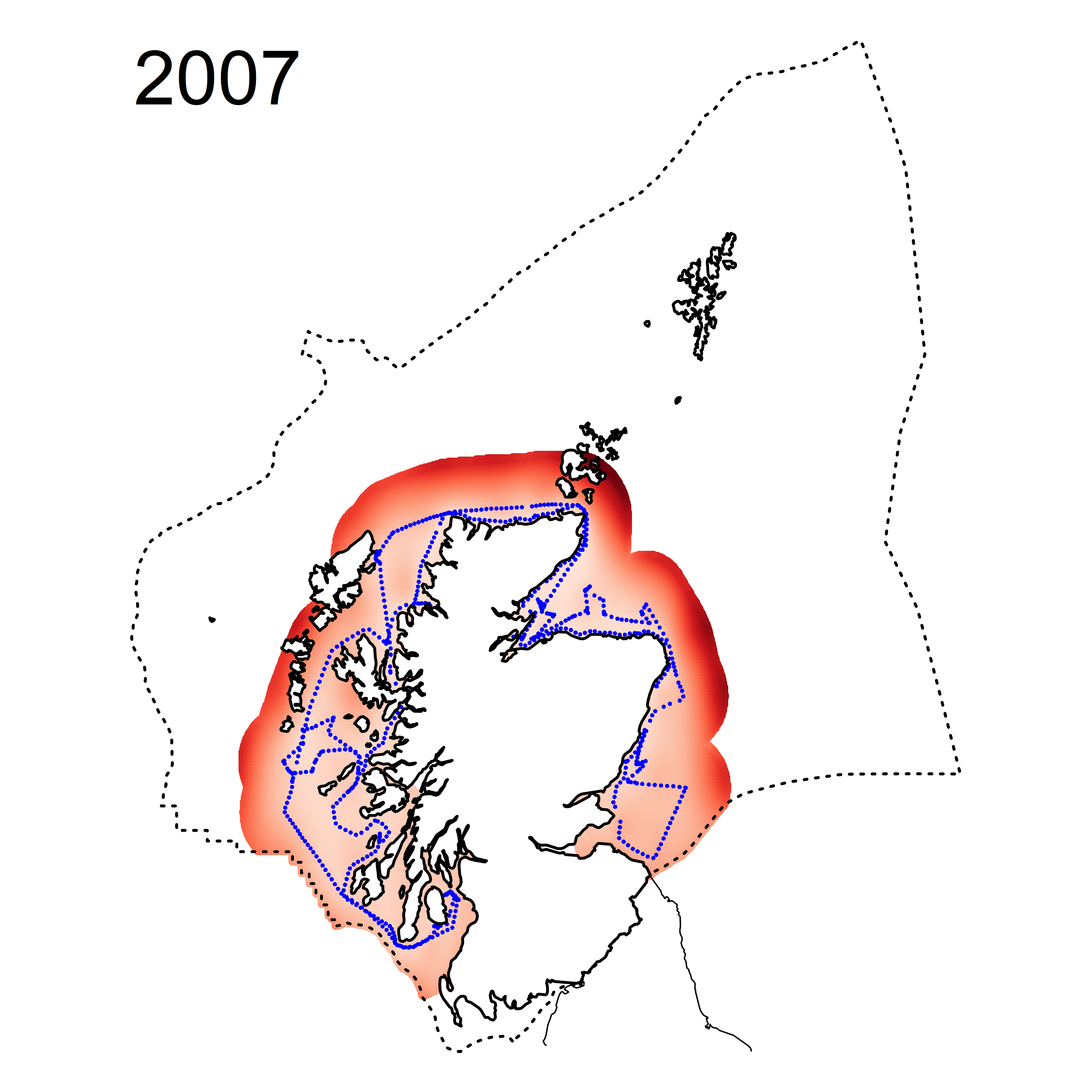
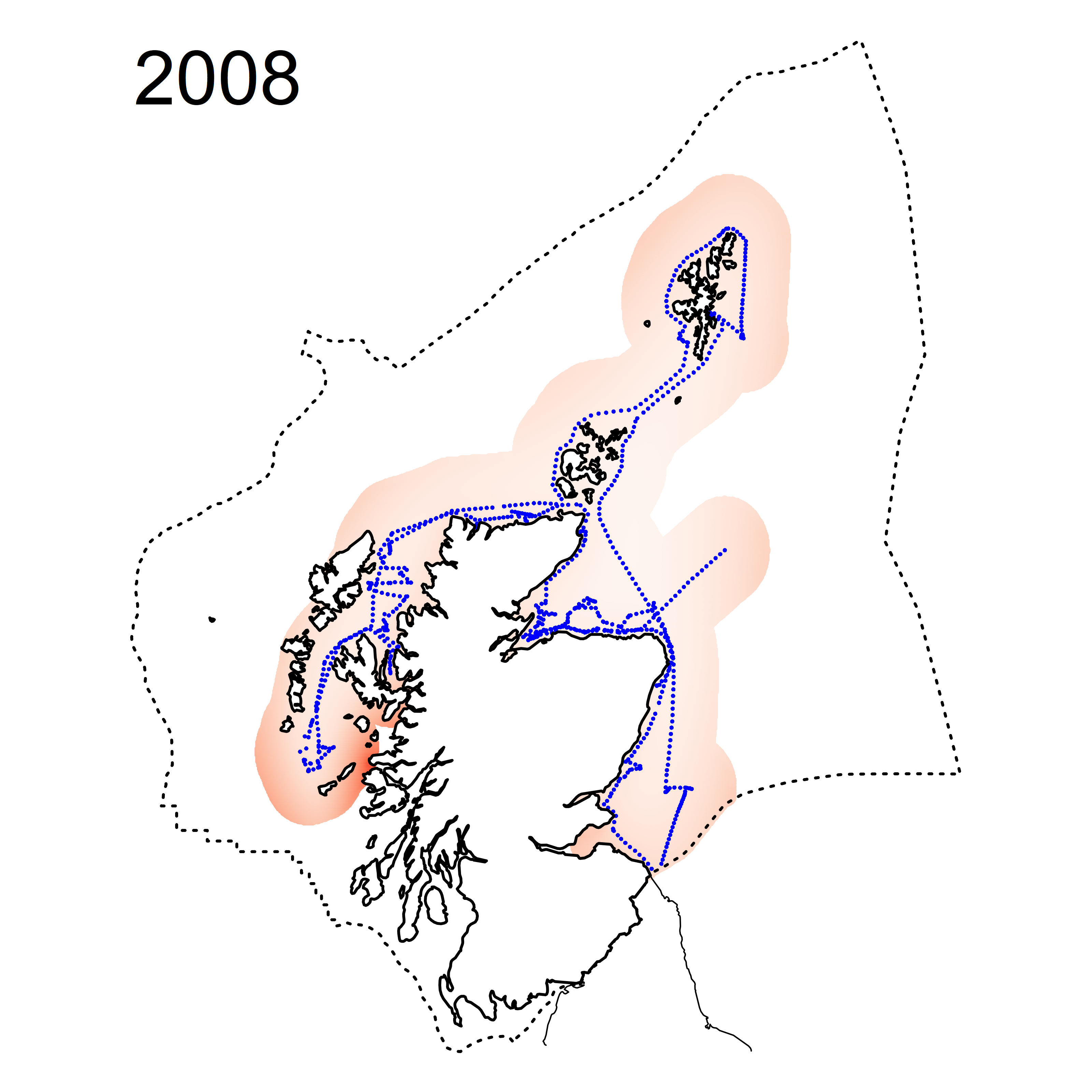
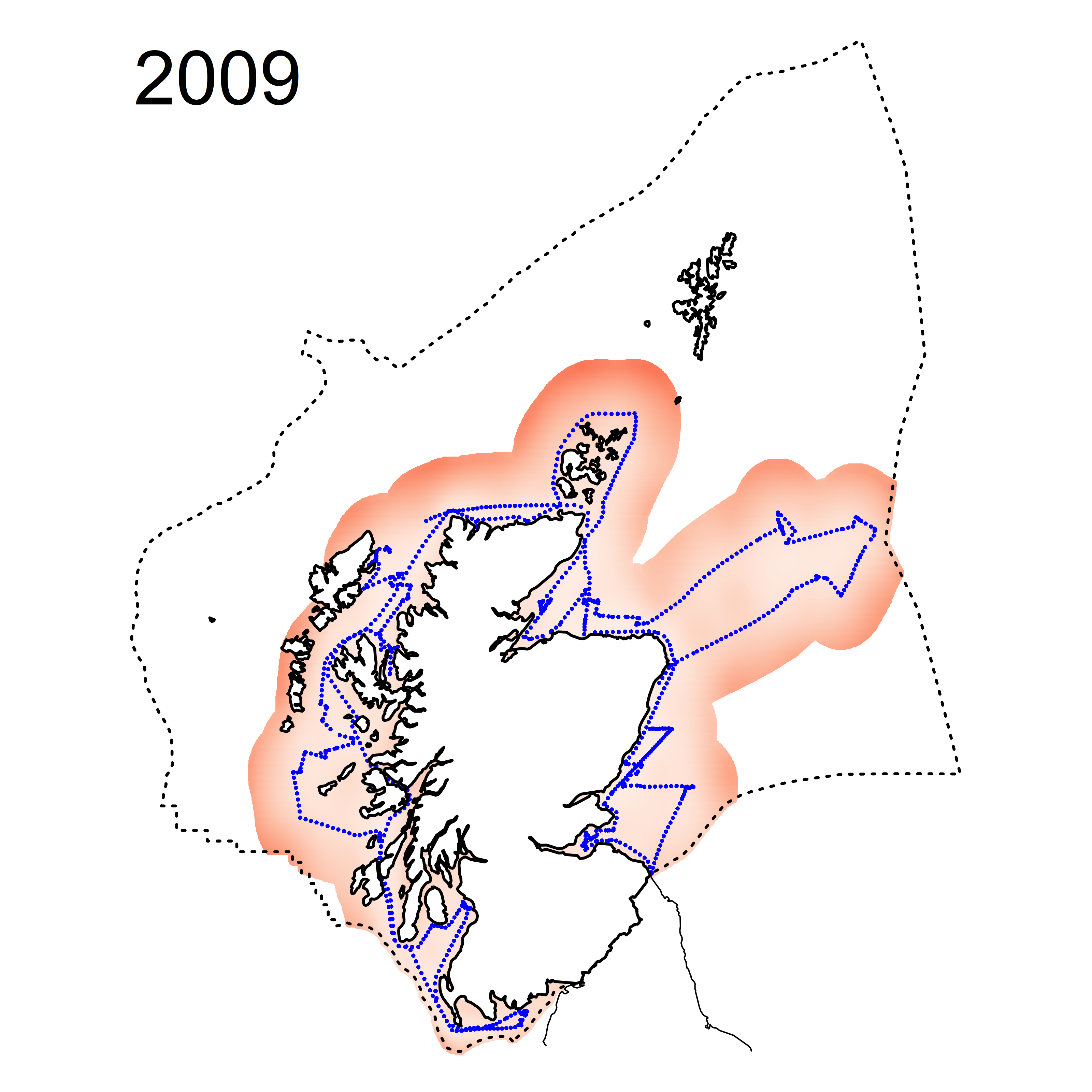
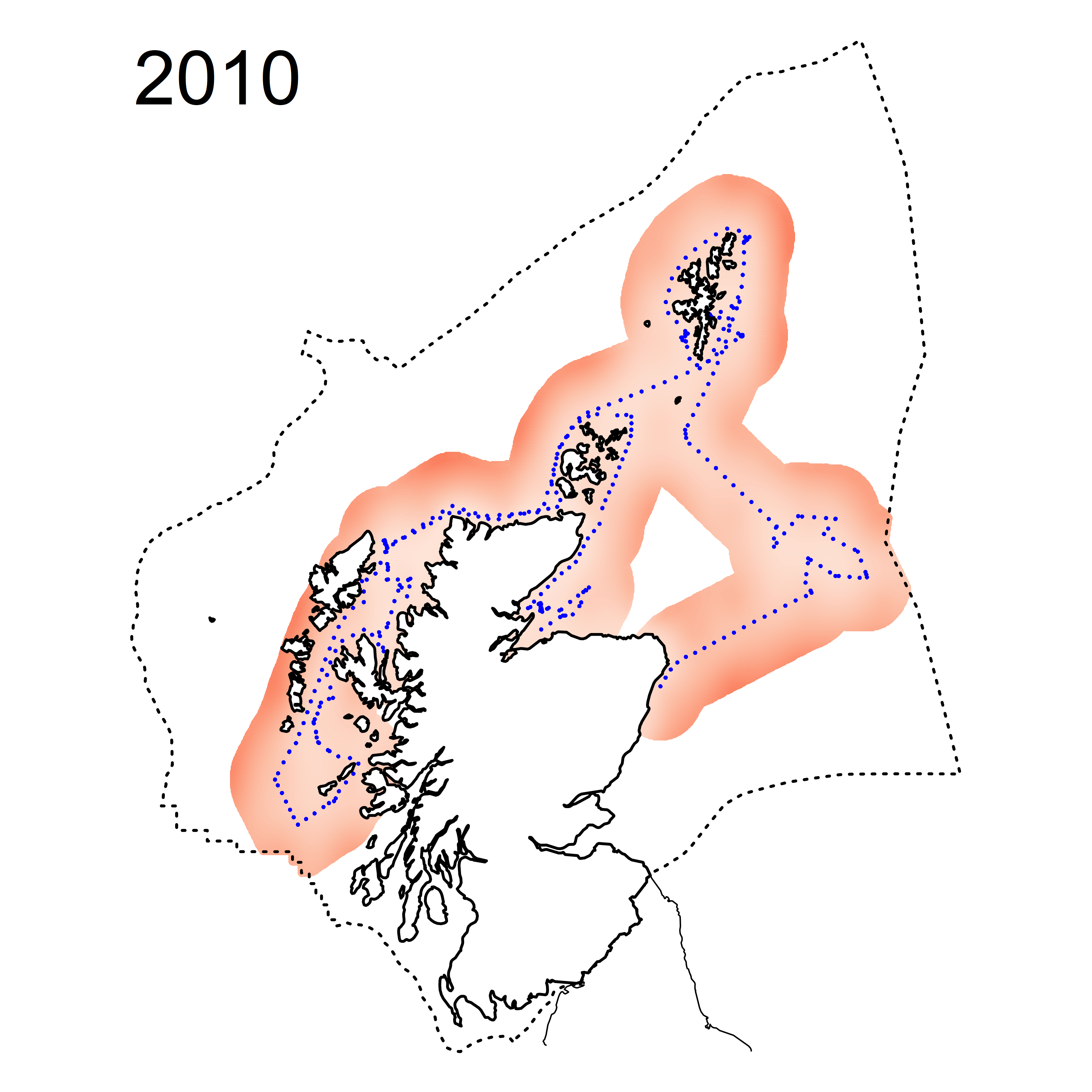
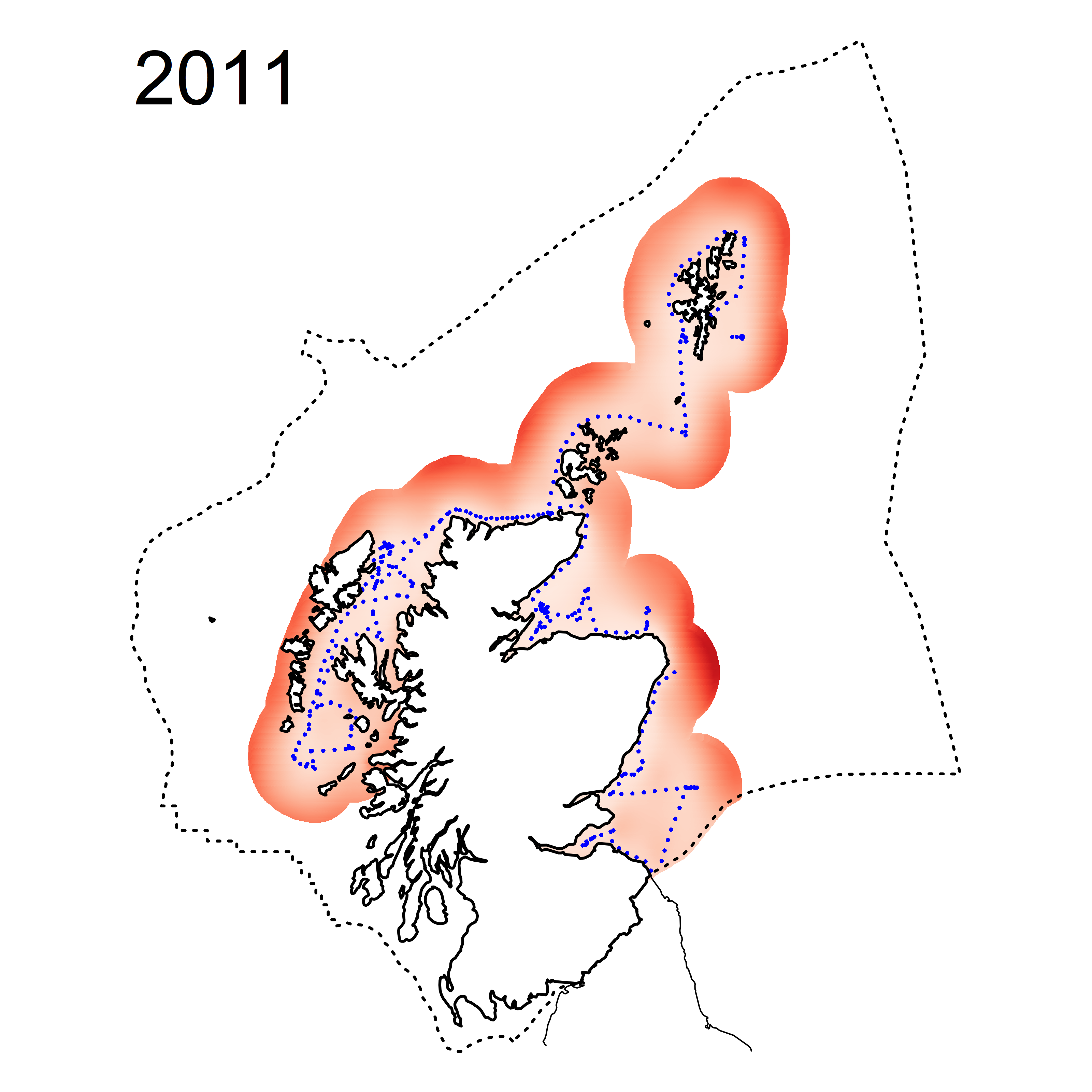
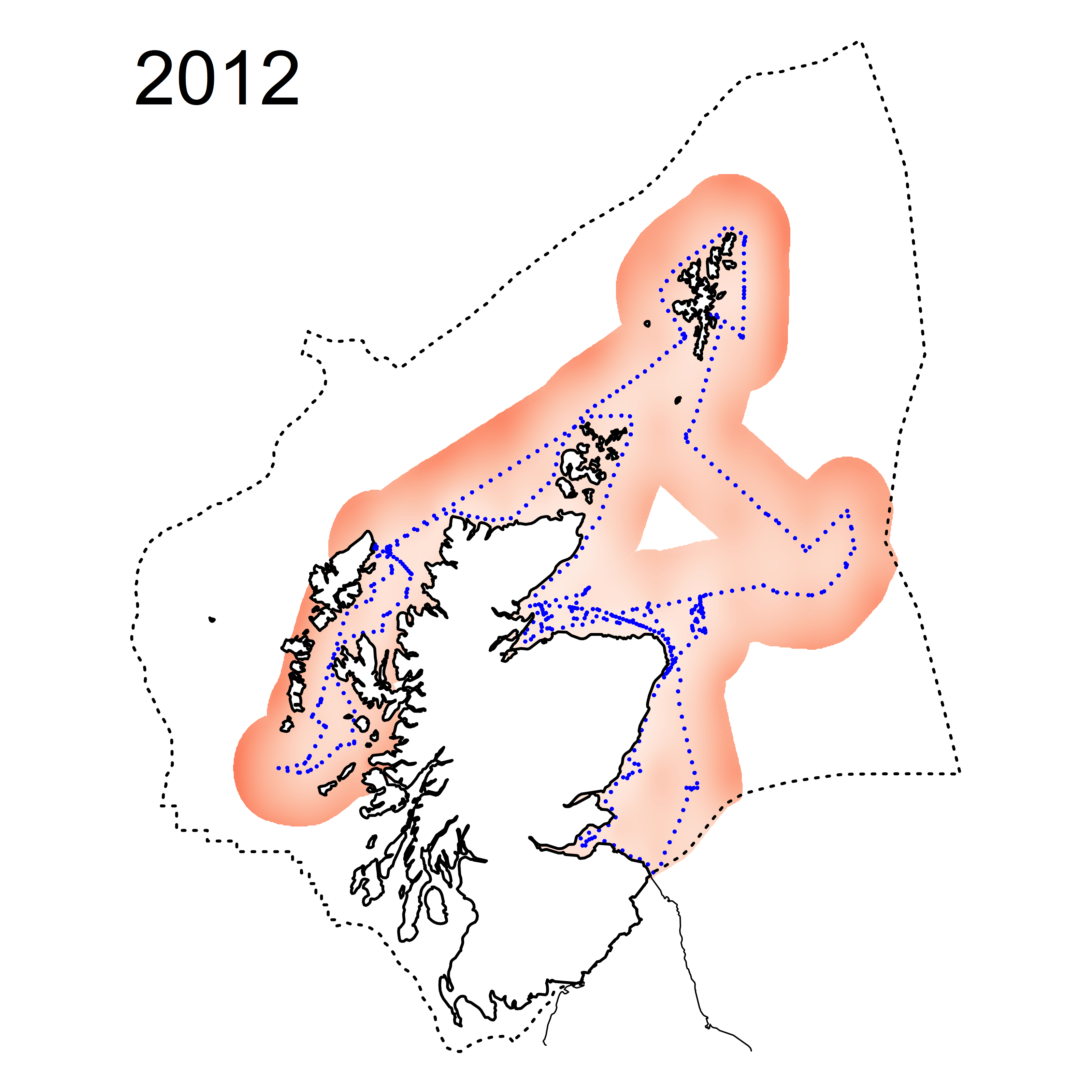
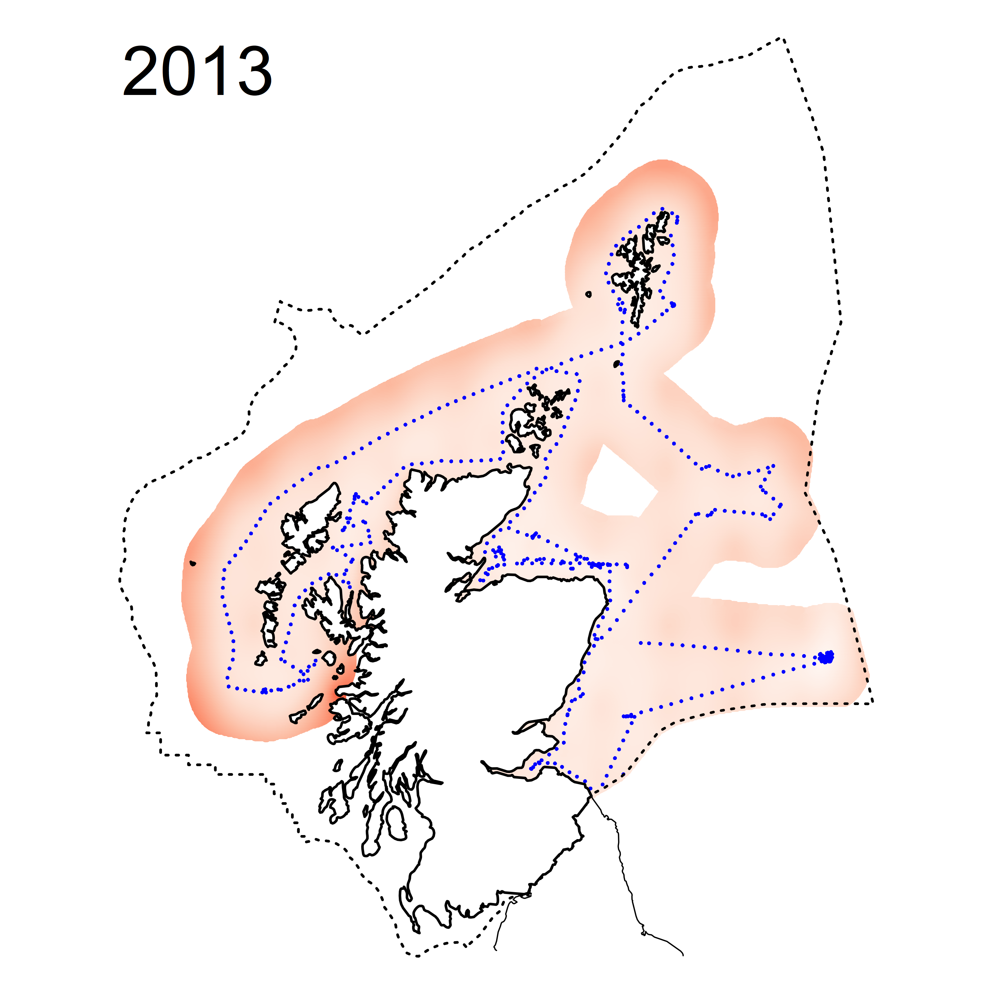
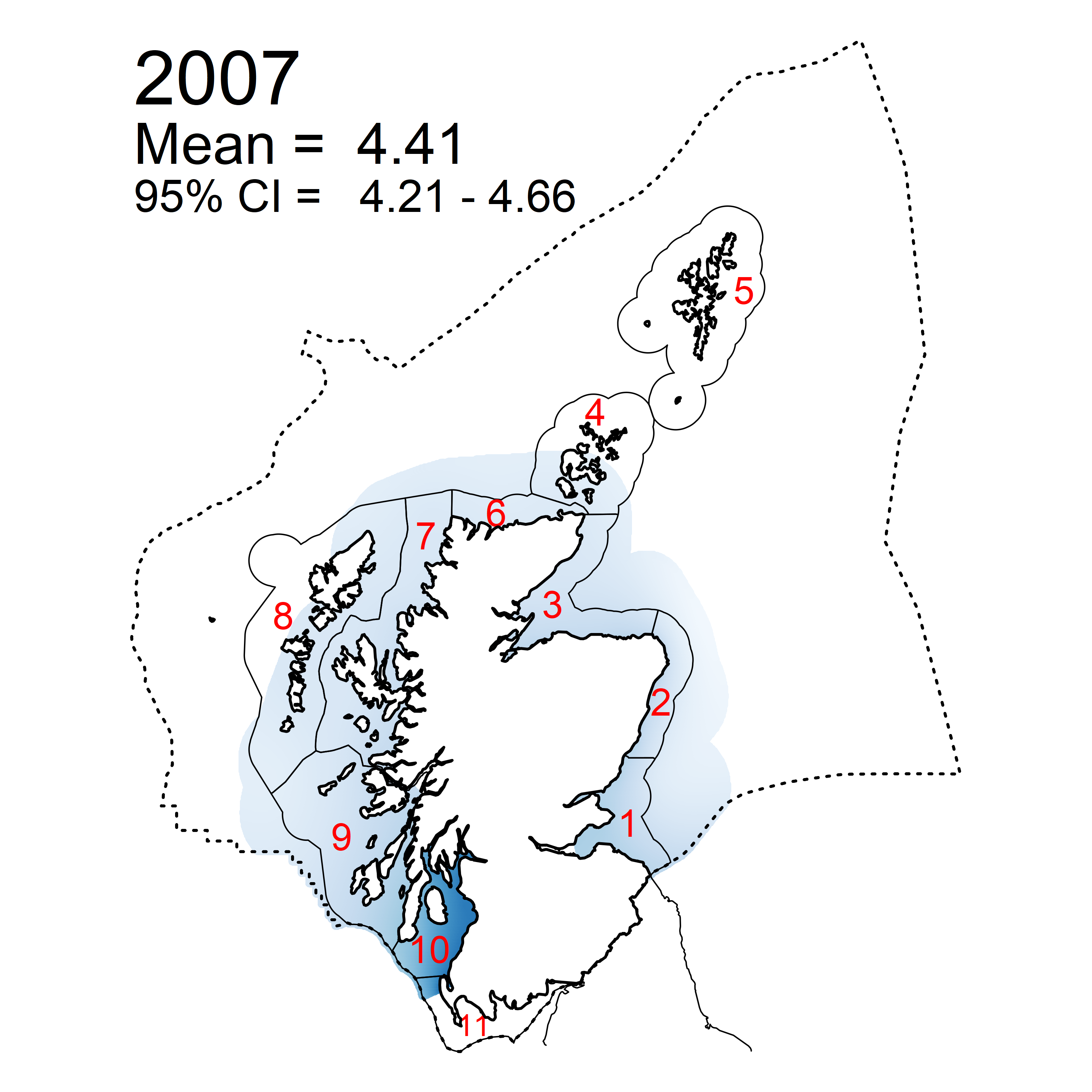
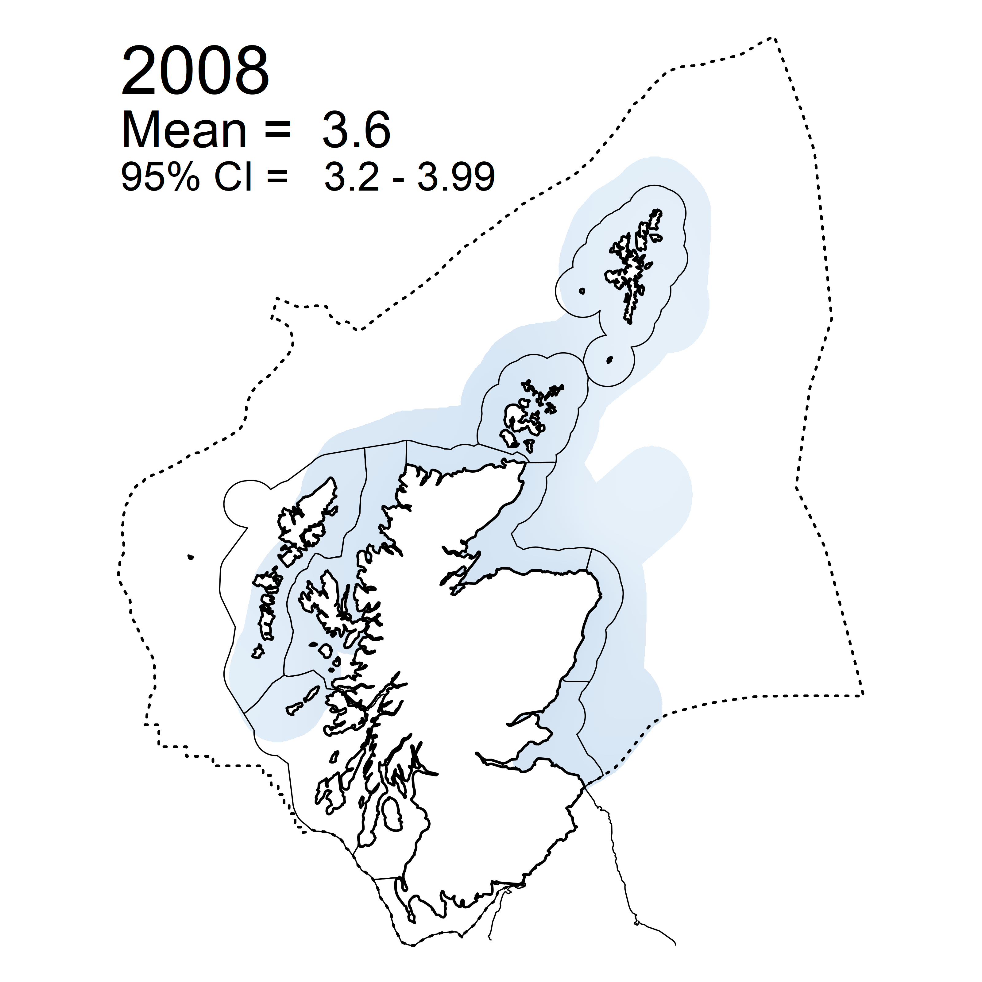
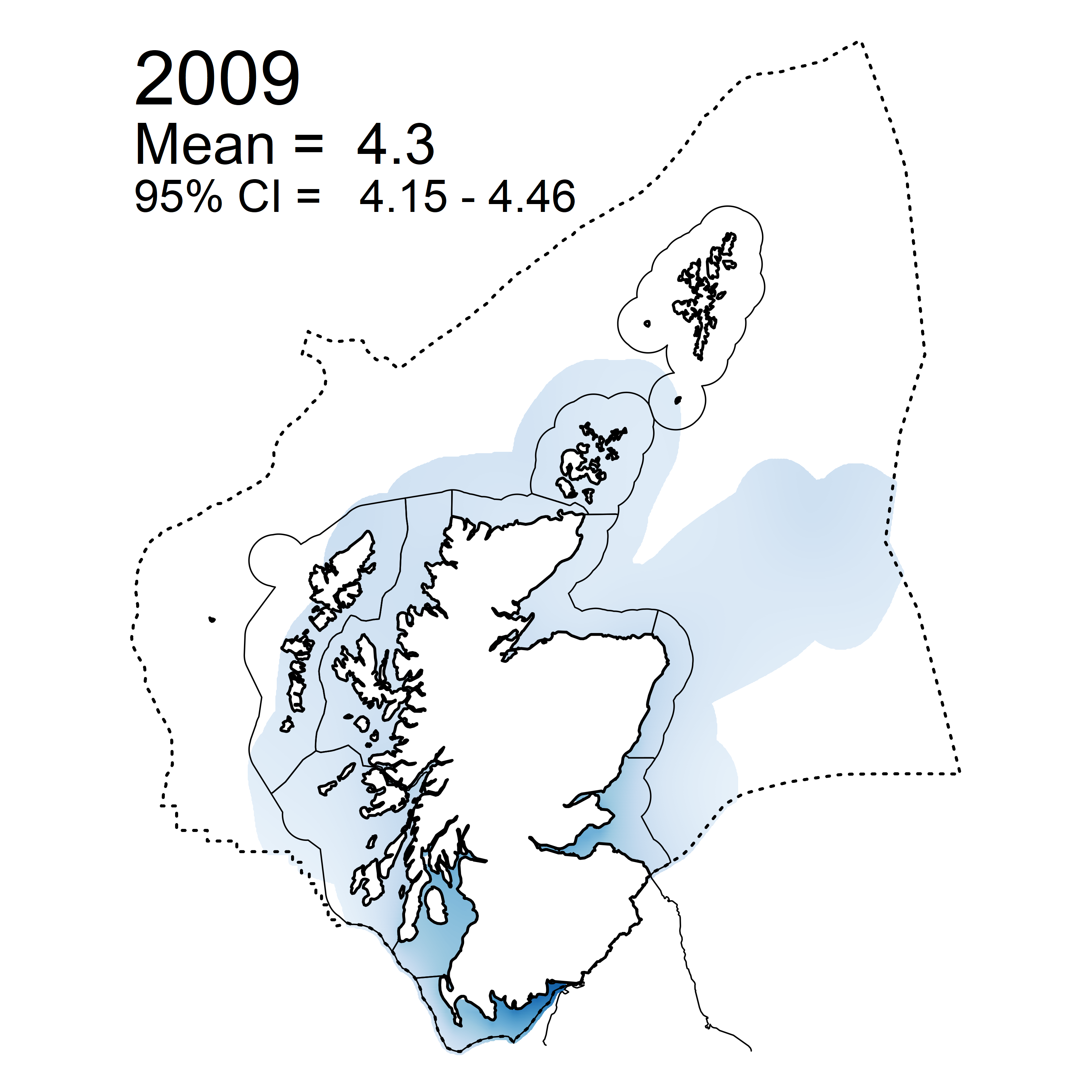
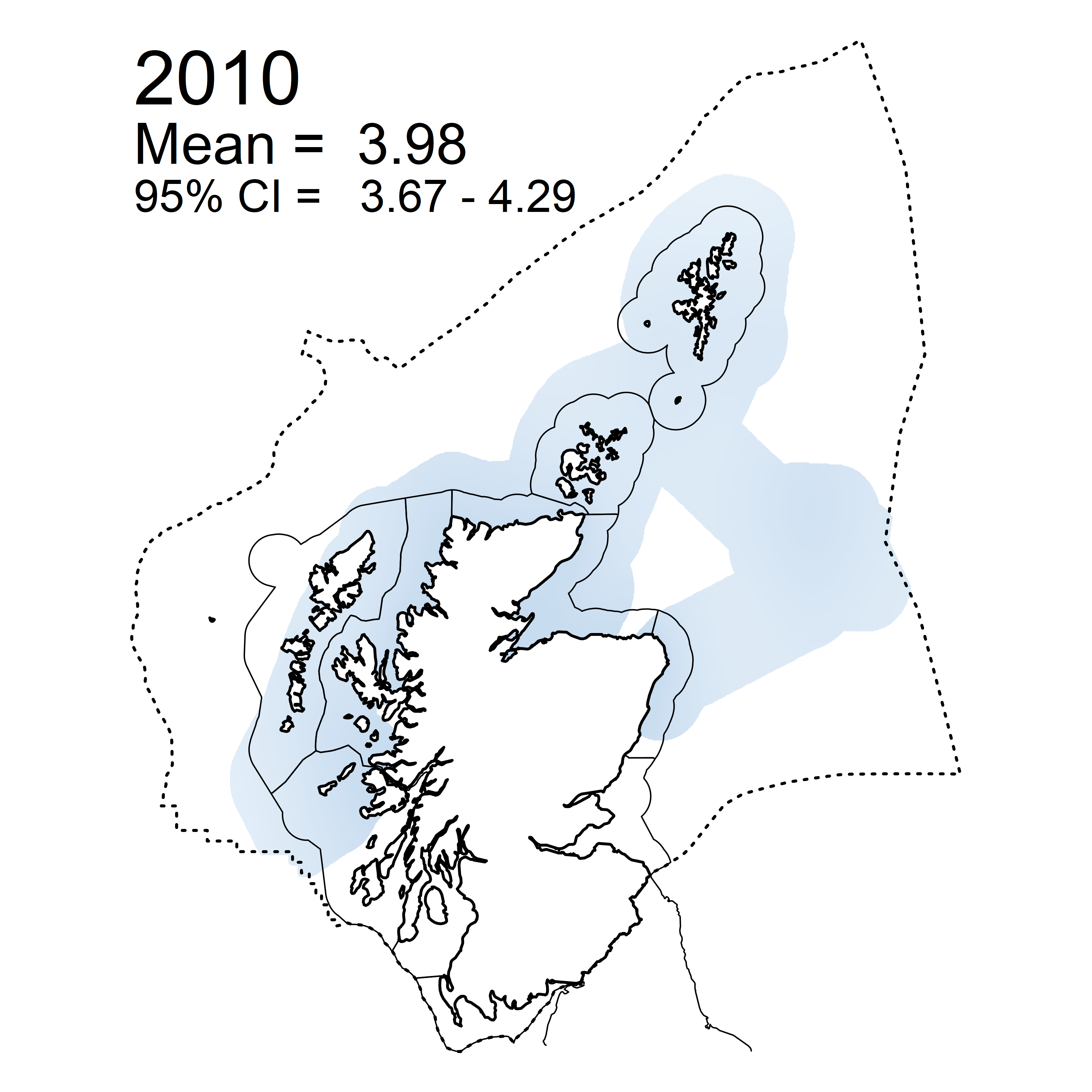
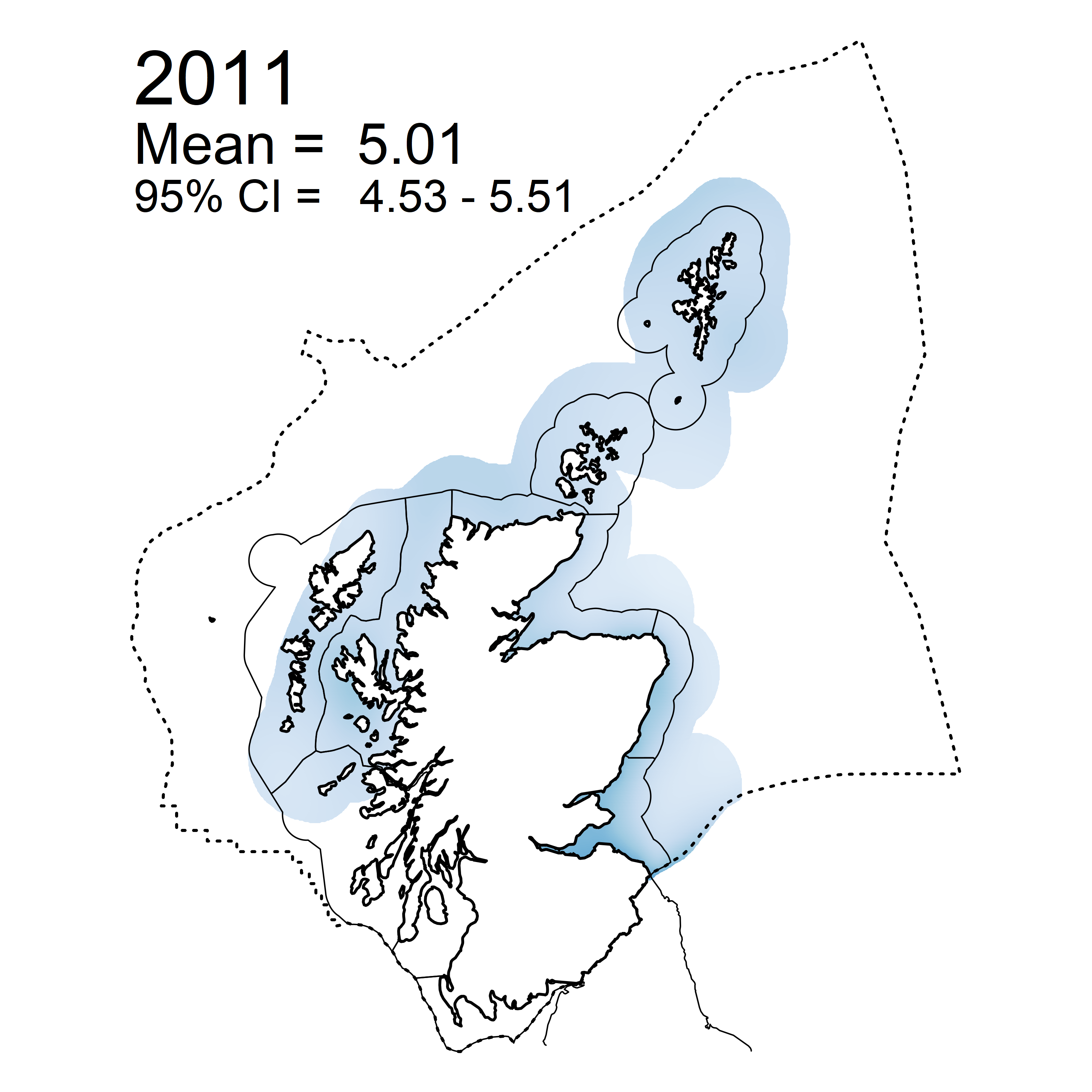
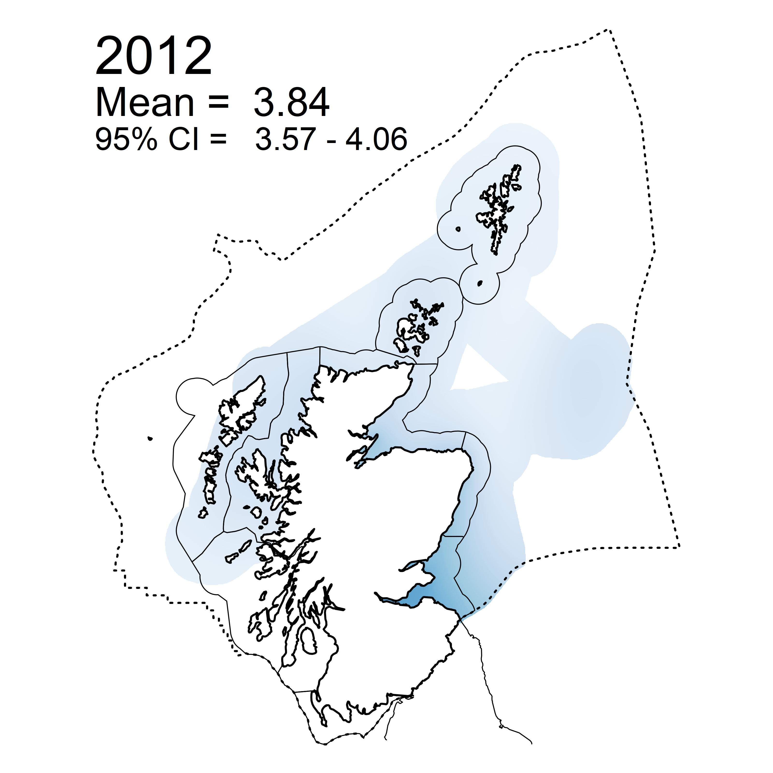
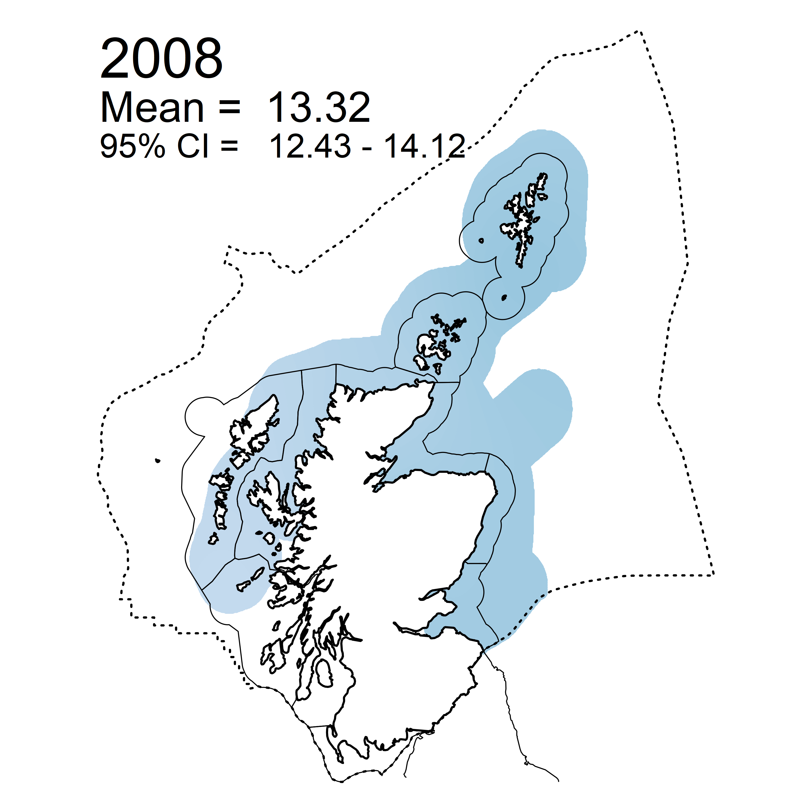
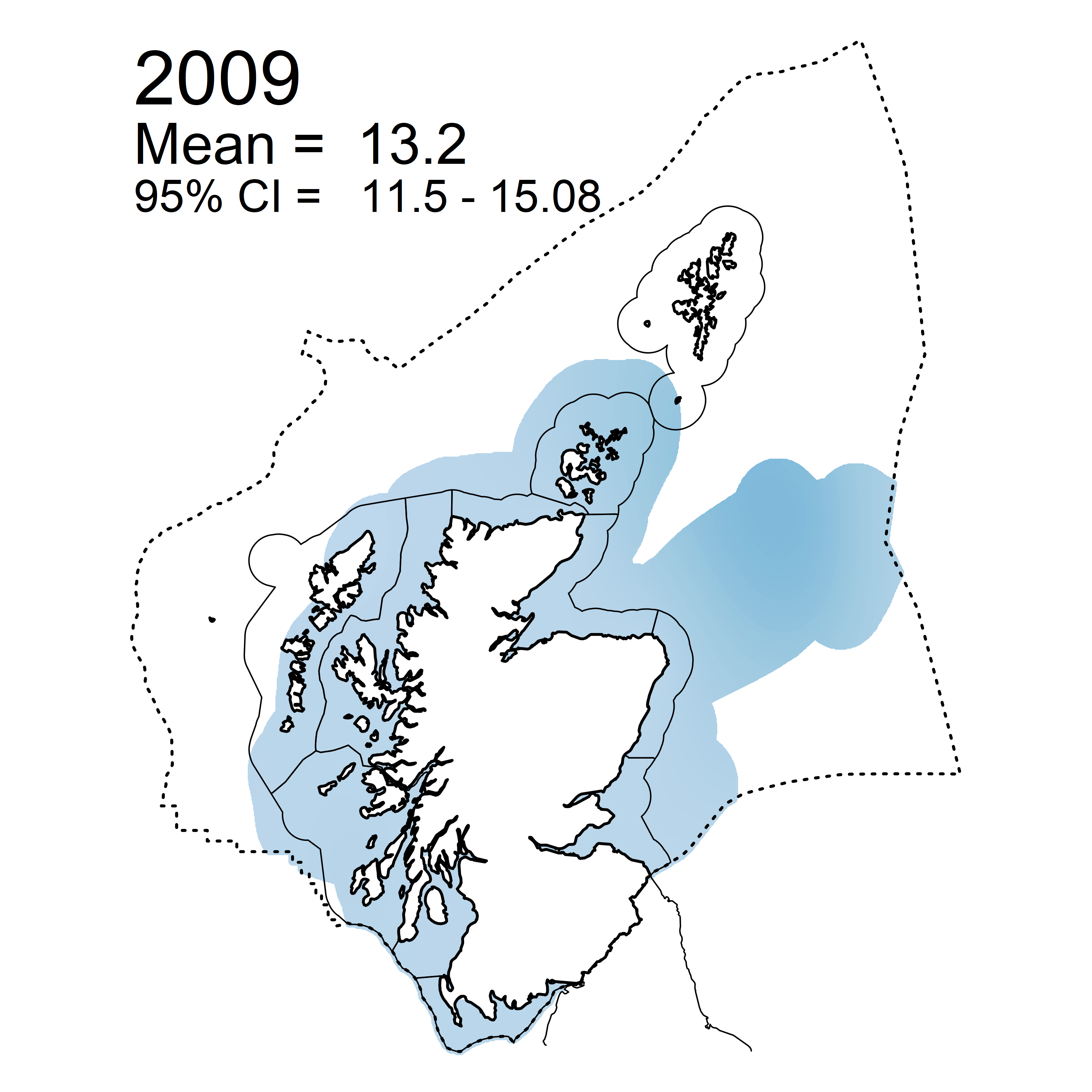
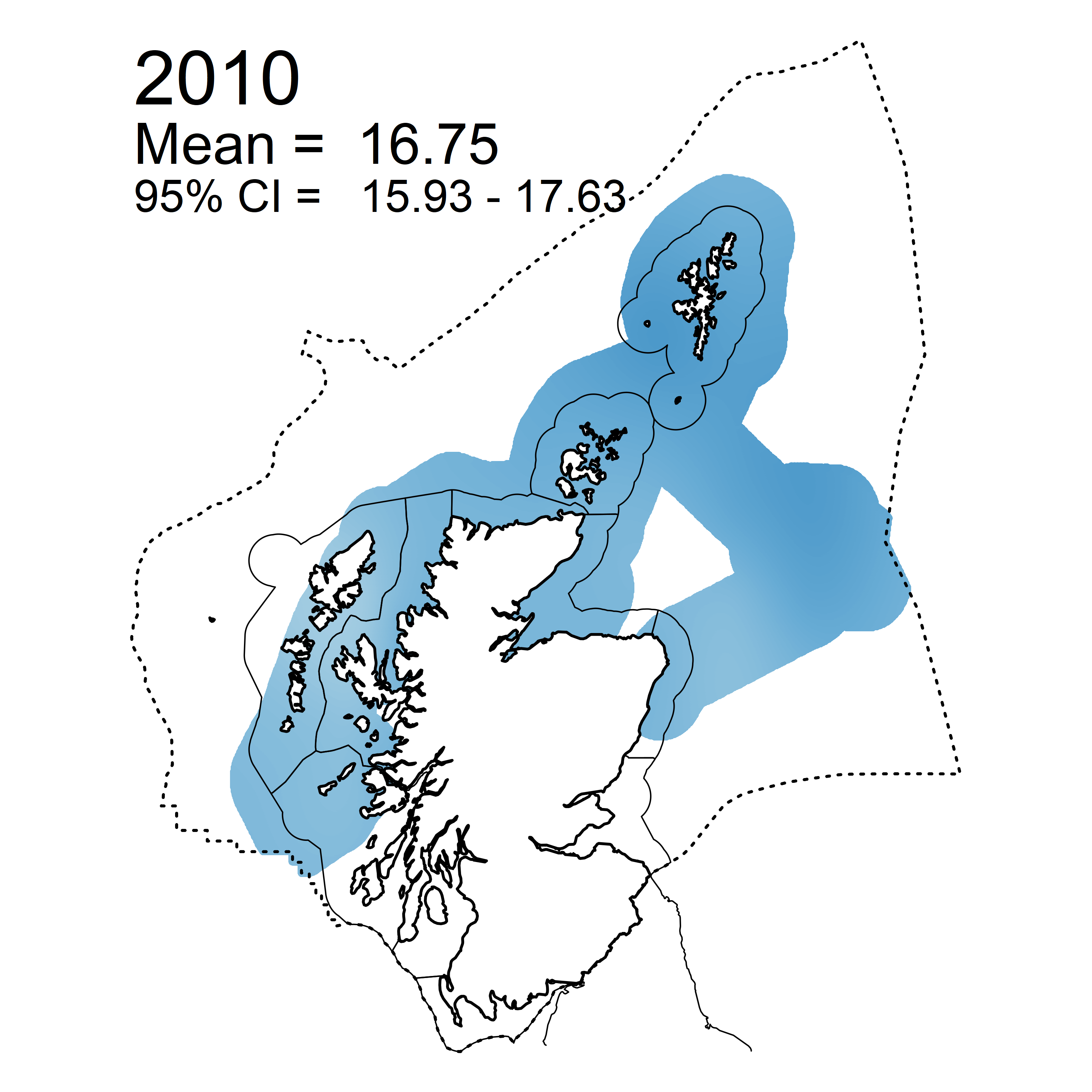
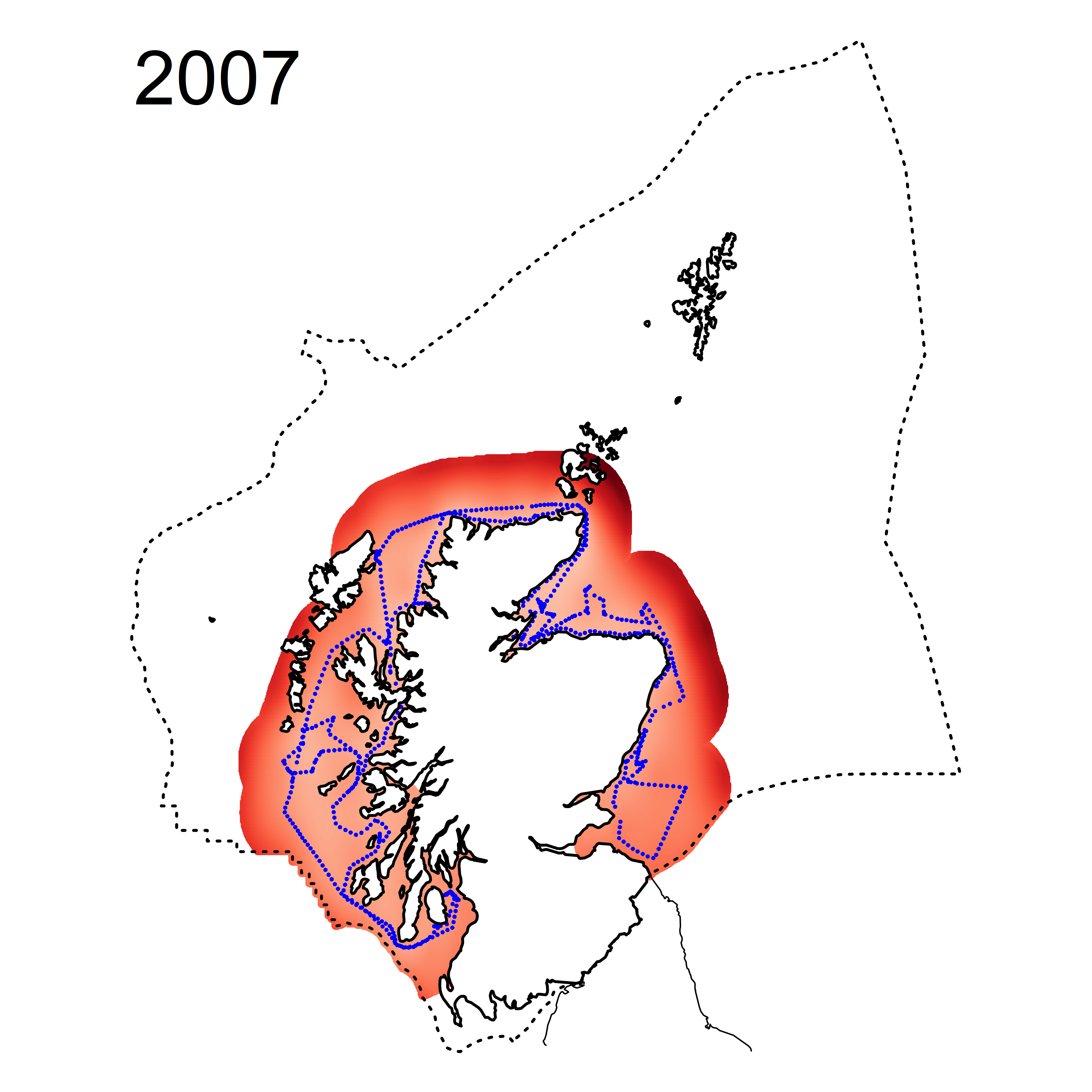
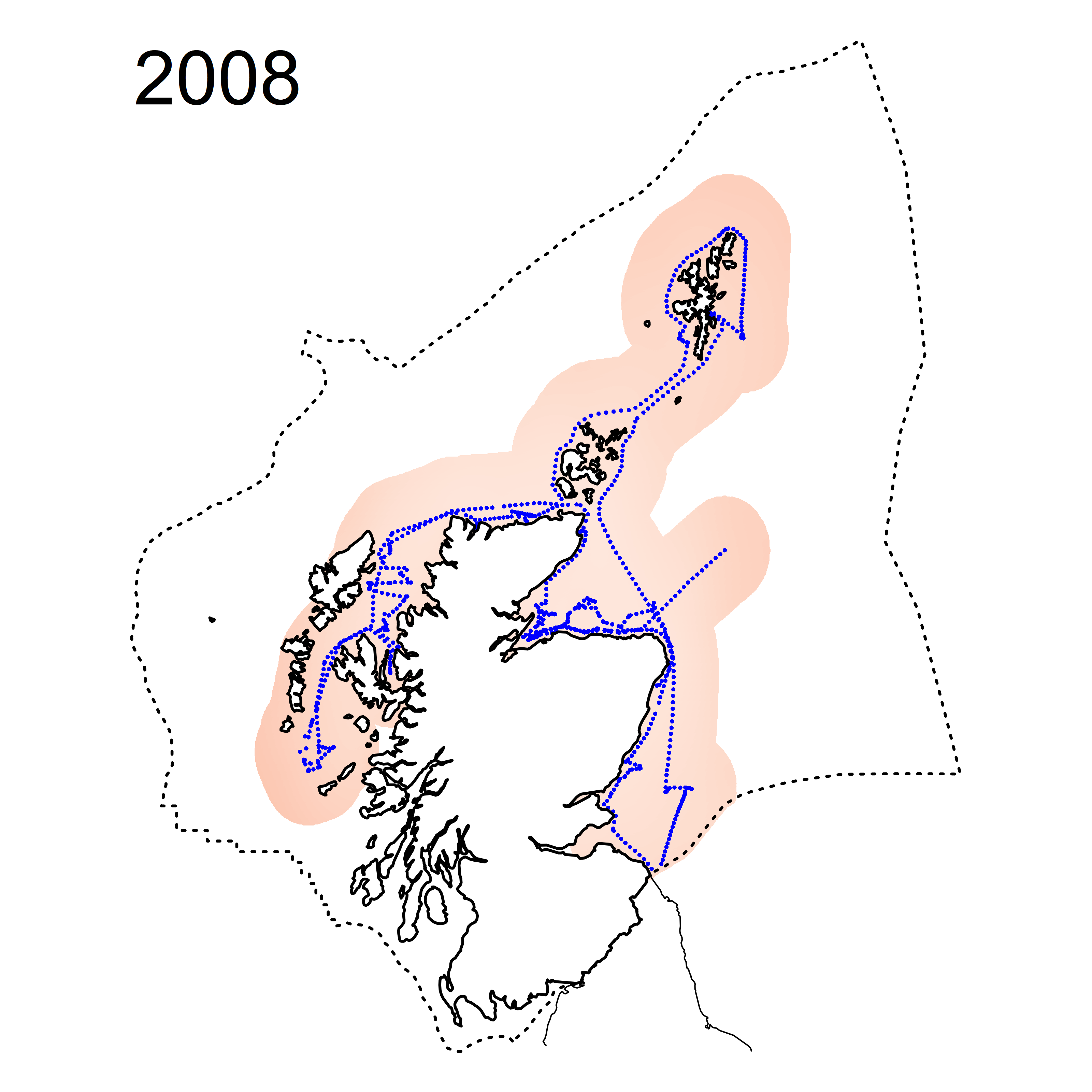
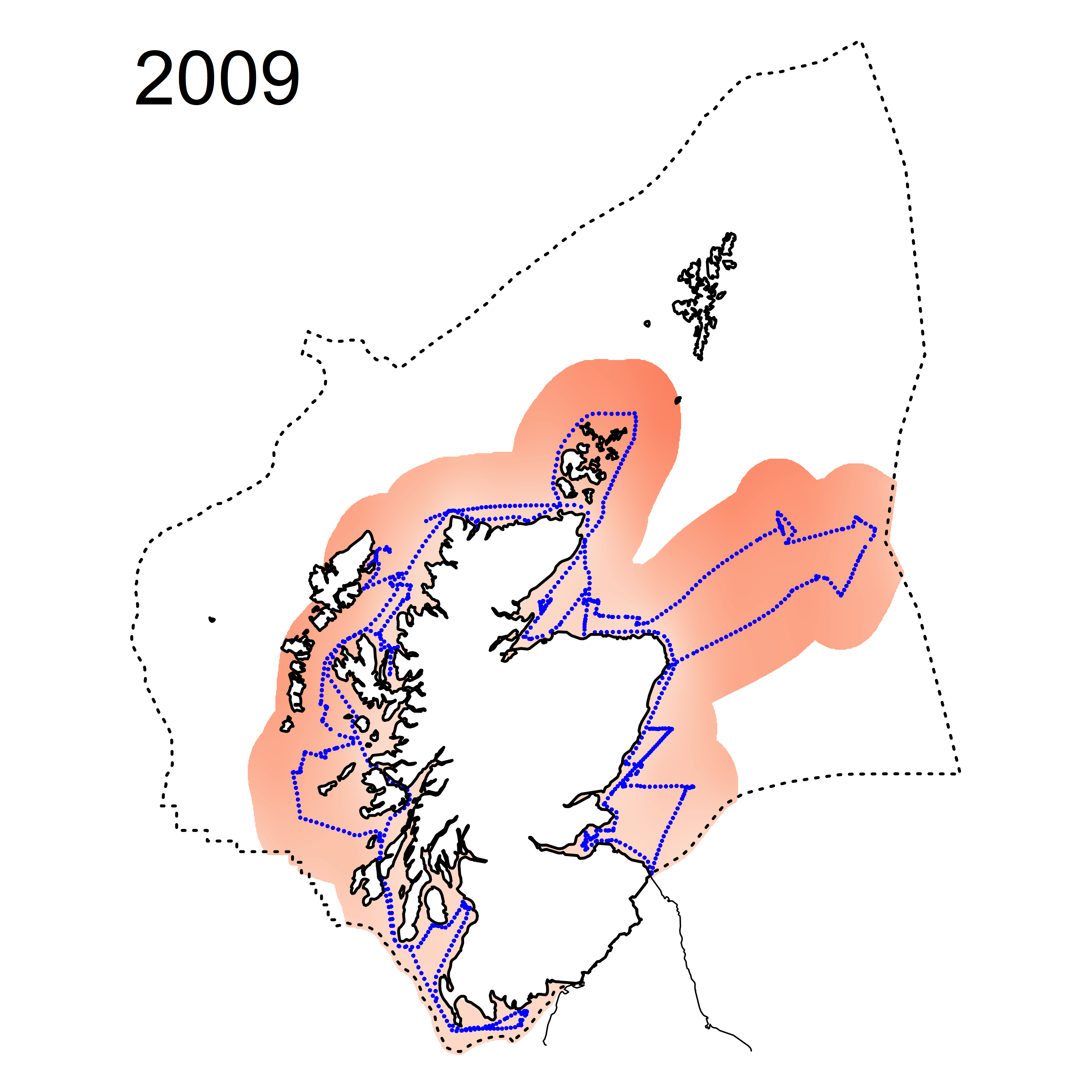
There is no specific ECoQO for TOxN but, as the ammonia contribution in Scottish waters is negligible, TOxN can be used as a proxy for DIN. Annual predicted normalised TOxN concentration for the entire assessment area ranged from 6.49 µM in 2007 to 9.93 µM in 2010 (Figure b). It is cautioned that the precision of the model decreases as it reaches the bounds of modelled area as presented in the CV% plot for normalised TOxN (Figure c).

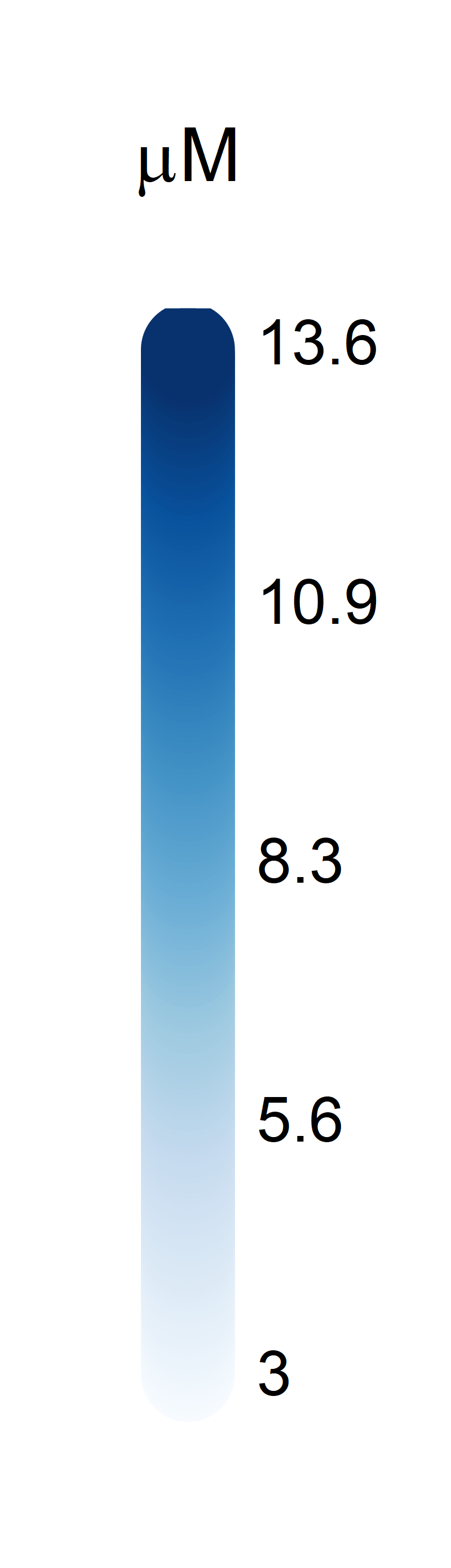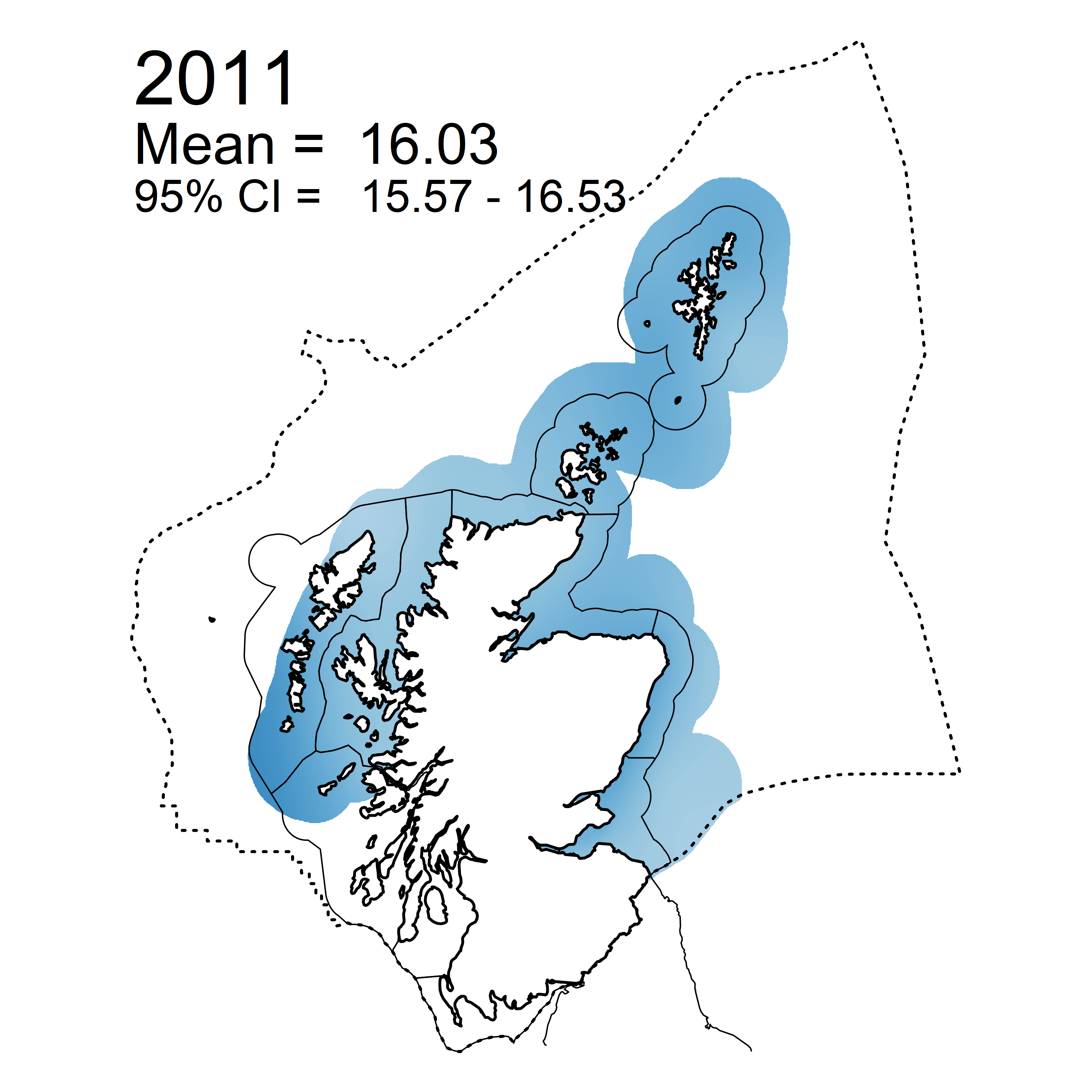
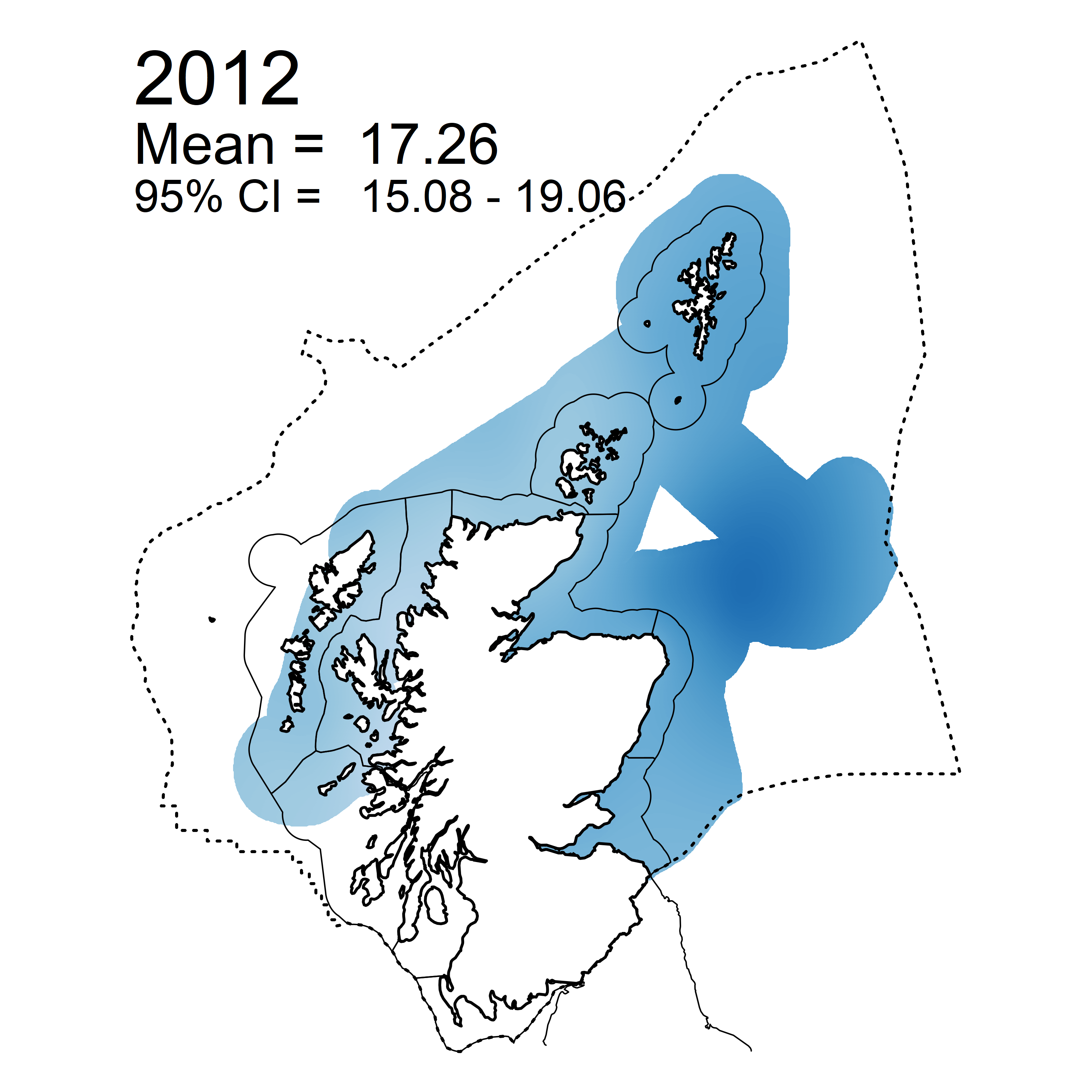
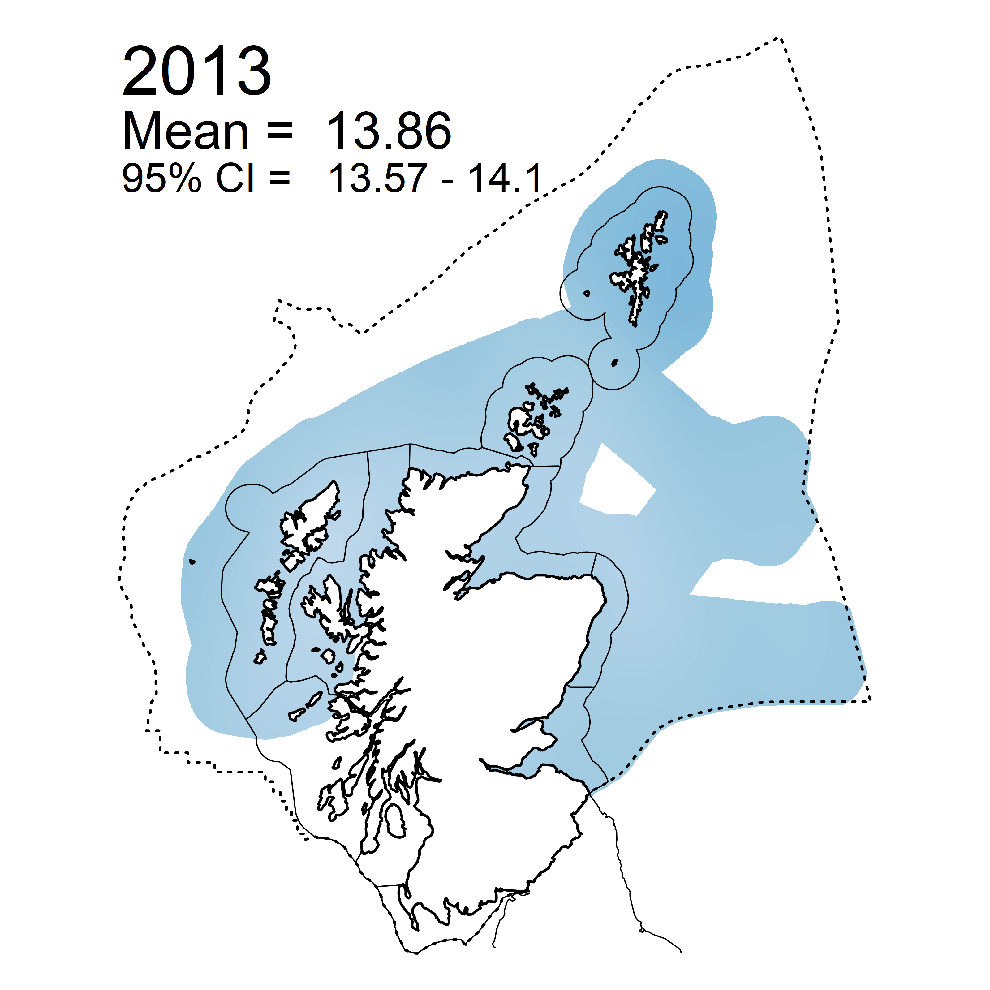
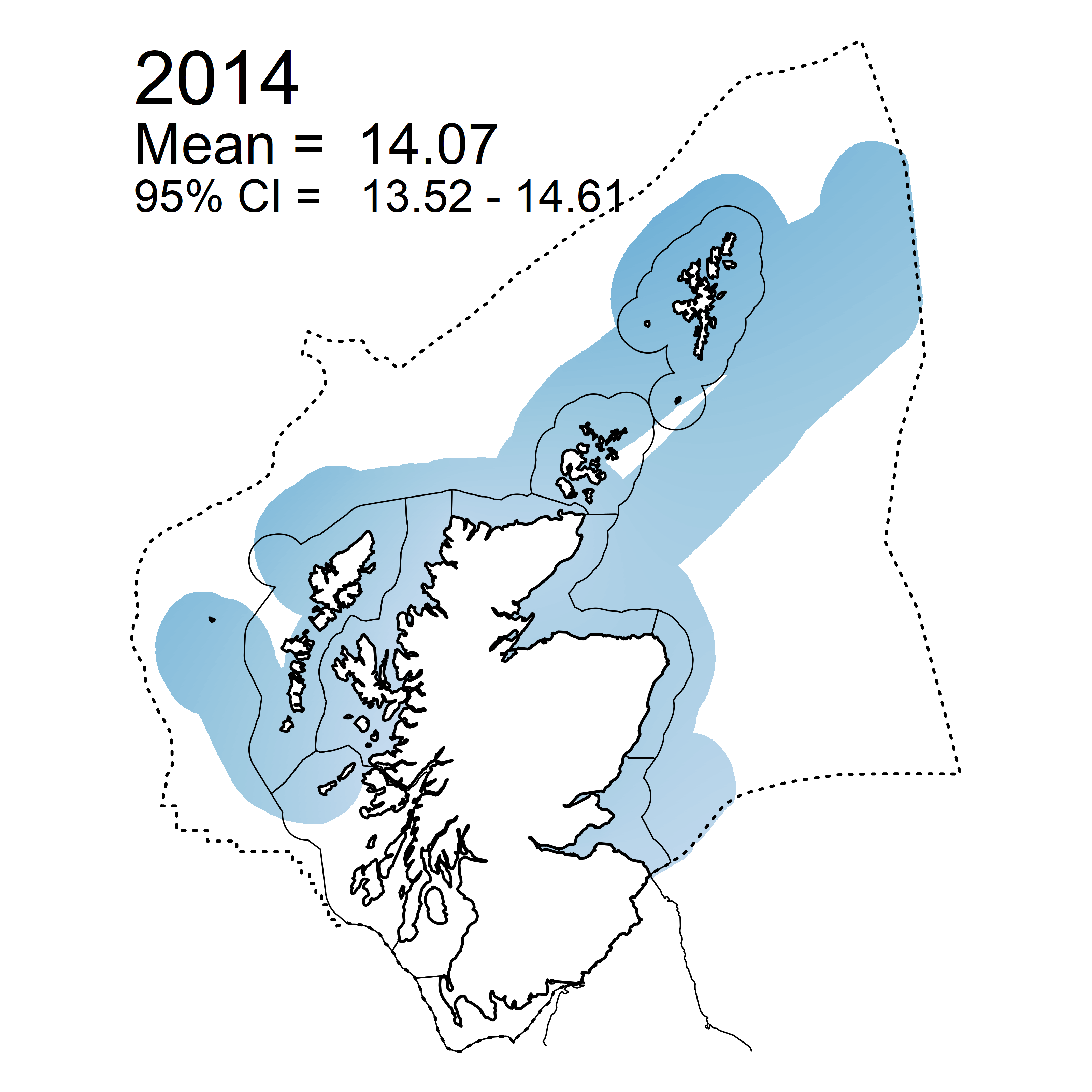
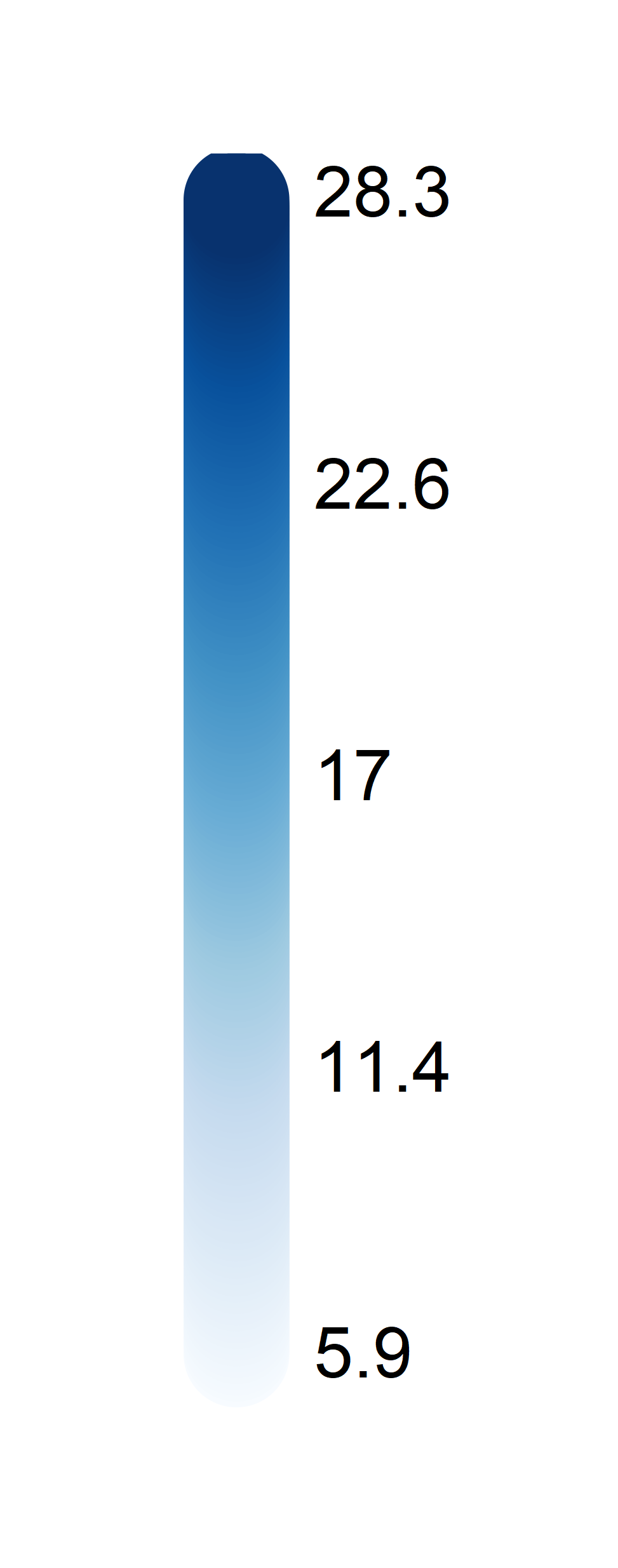
Figure b: Mean predicted salinity normalised TOxN concentrations (µM) for winter periods 2007 - 2019 collected as part of the CSEMP annual monitoring cruise.

Figure c: Coefficient of variation (CV%) of the modelled data set for salinity normalised TOxN. With least accuracy found on the outer boundaries furthest from sampling position.

Across all SMRs the predicted mean winter TOxN concentrations (salinity normalised) were found to be below the elevated DIN EcoQOs (15 µM) for offshore waters (salinity >34.5), with concentrations in most SMRs also being below the background concentration (10 µM, offshore) (Figure b & d).

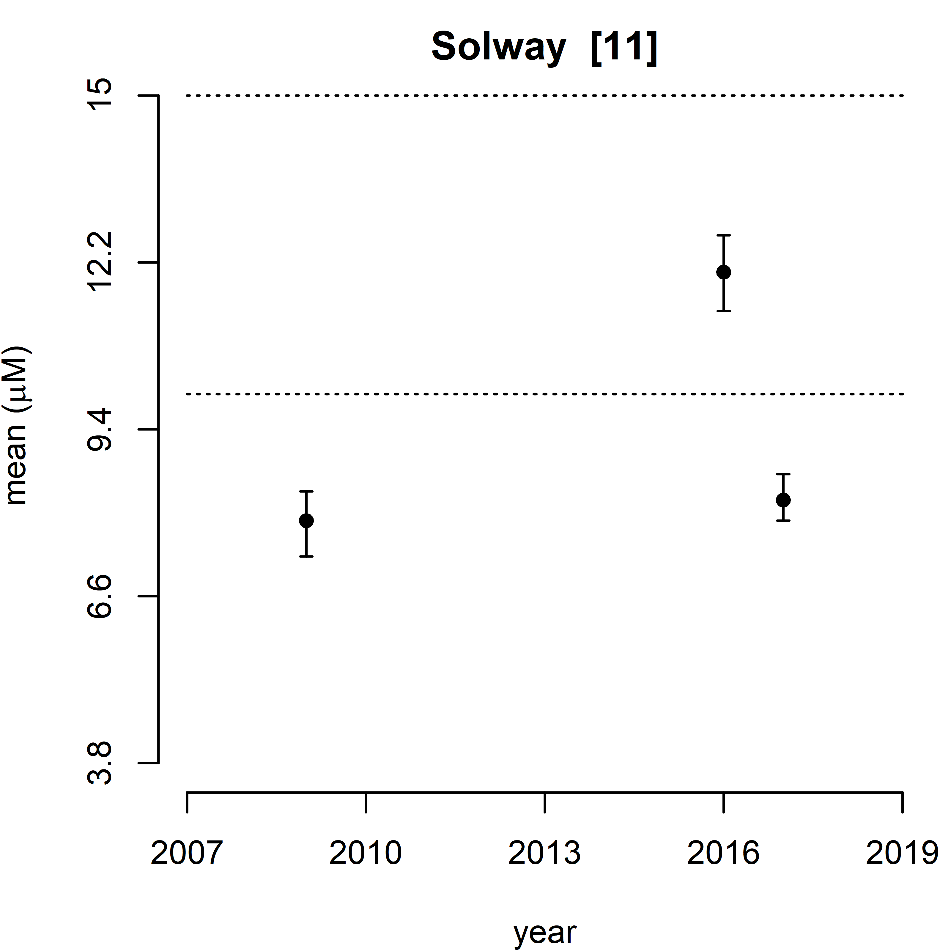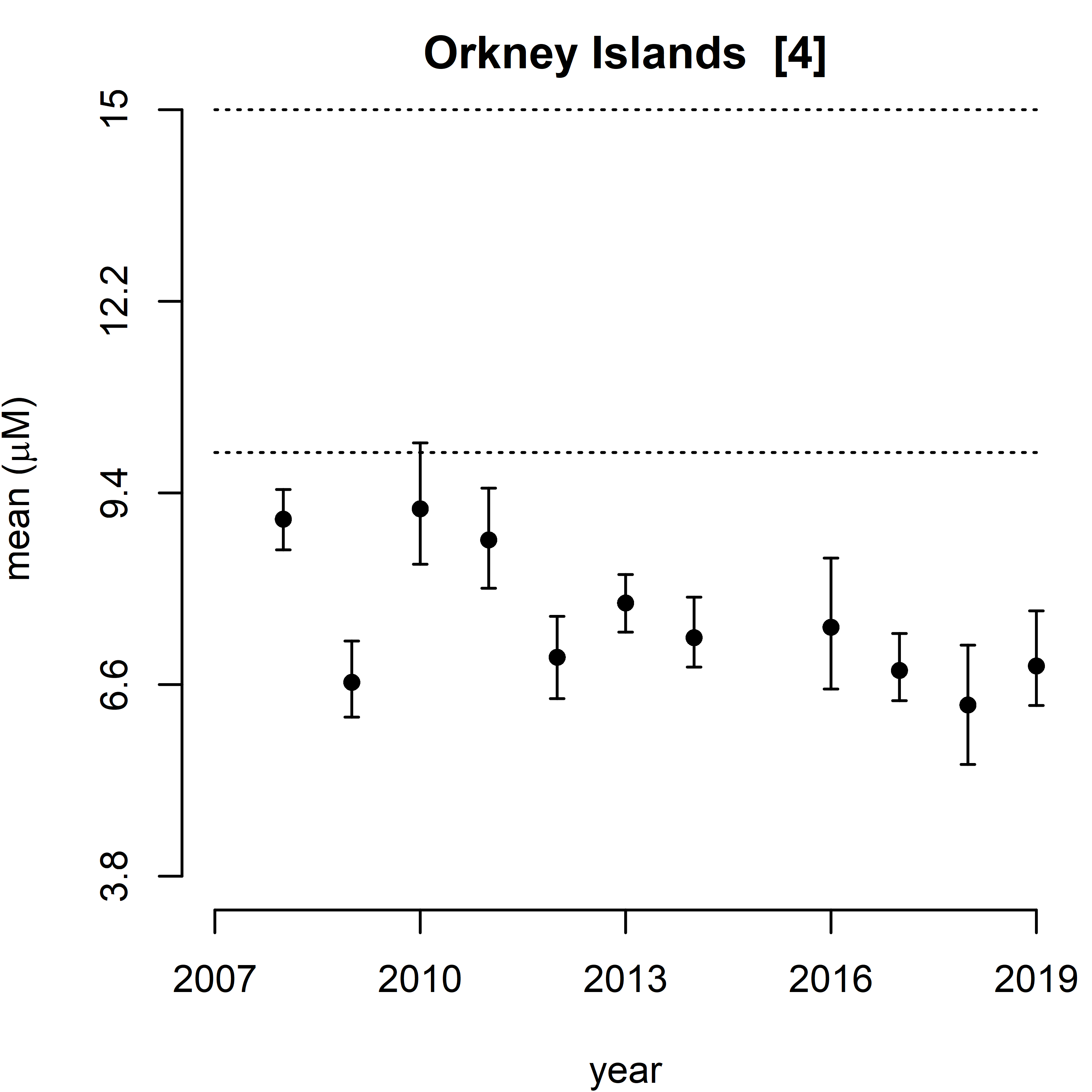
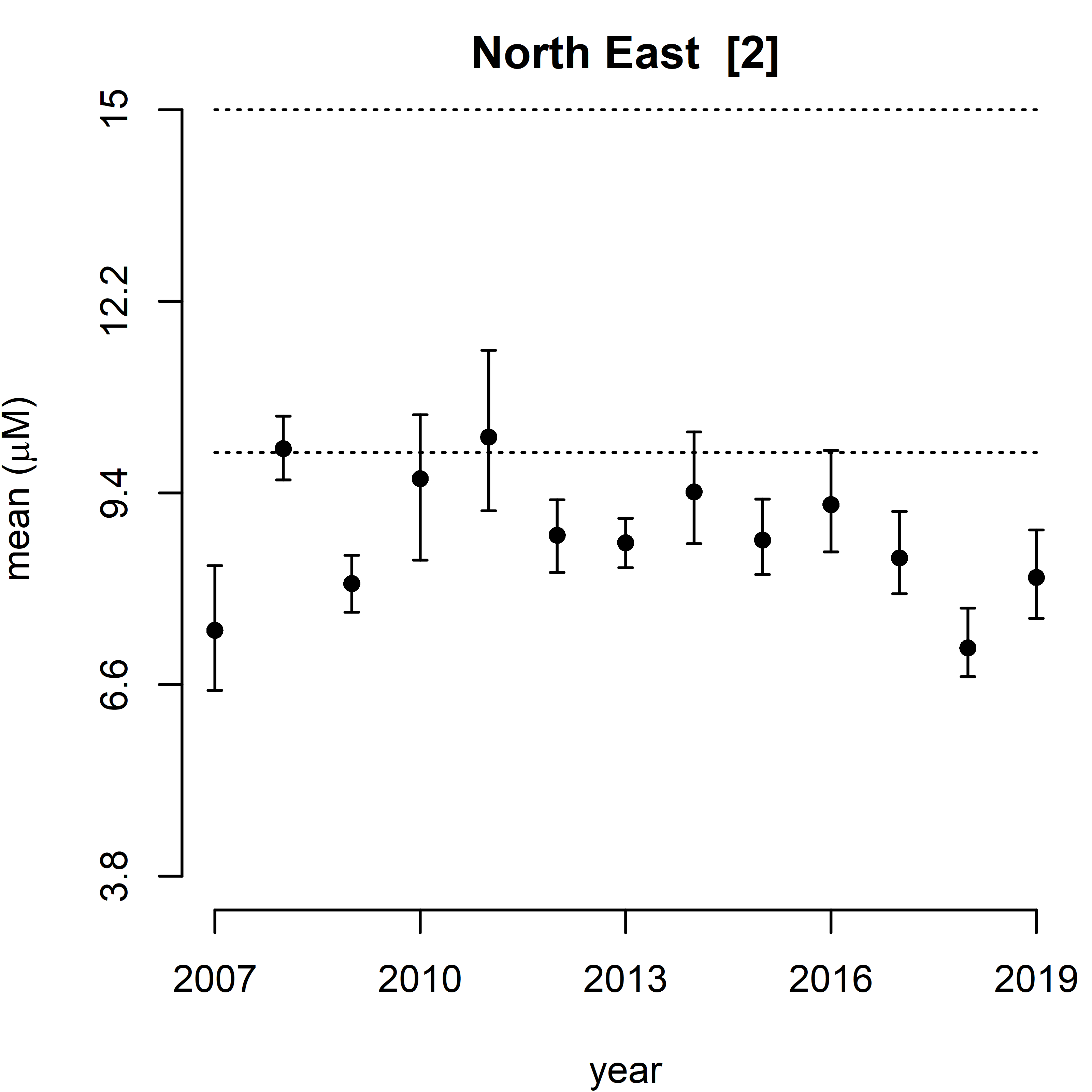
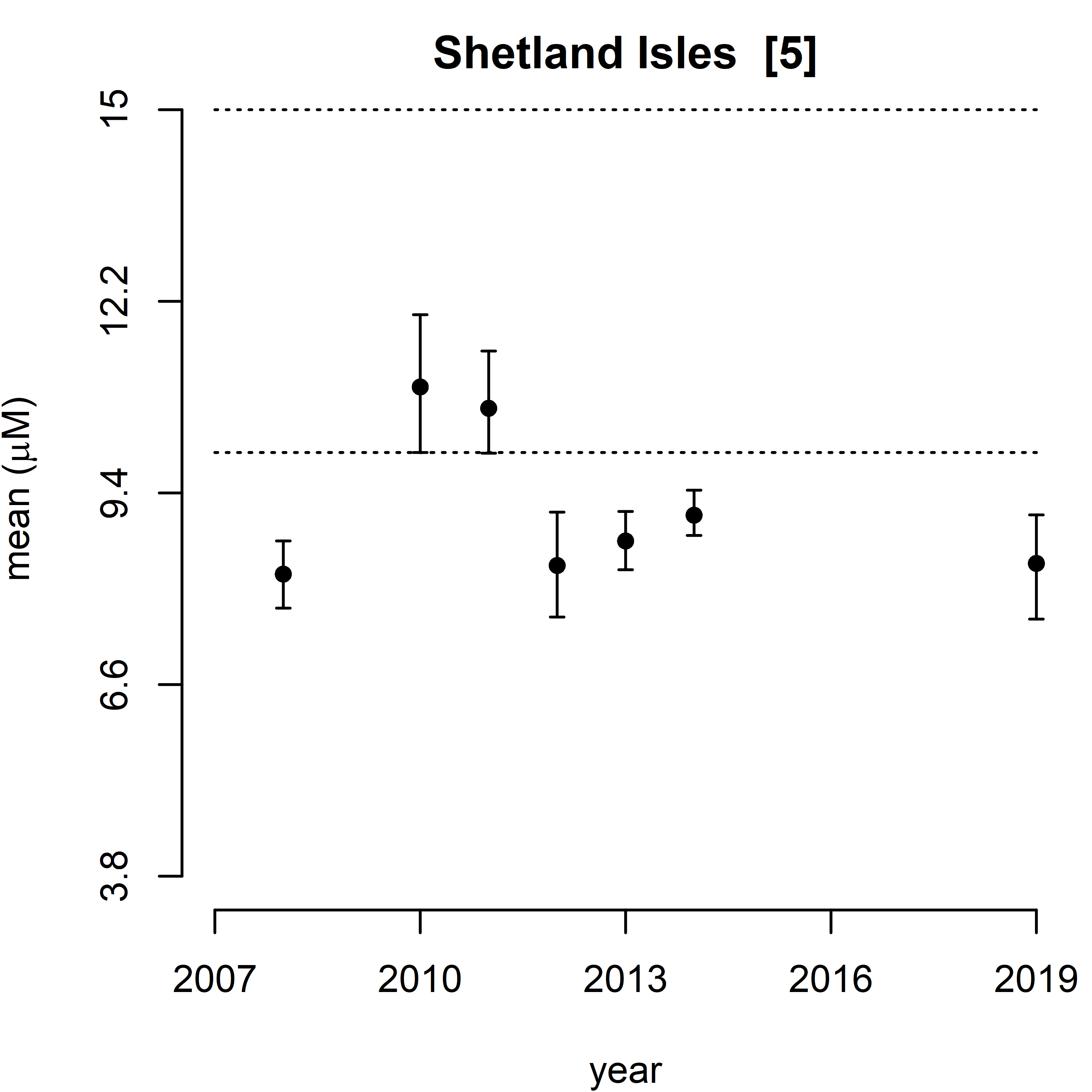
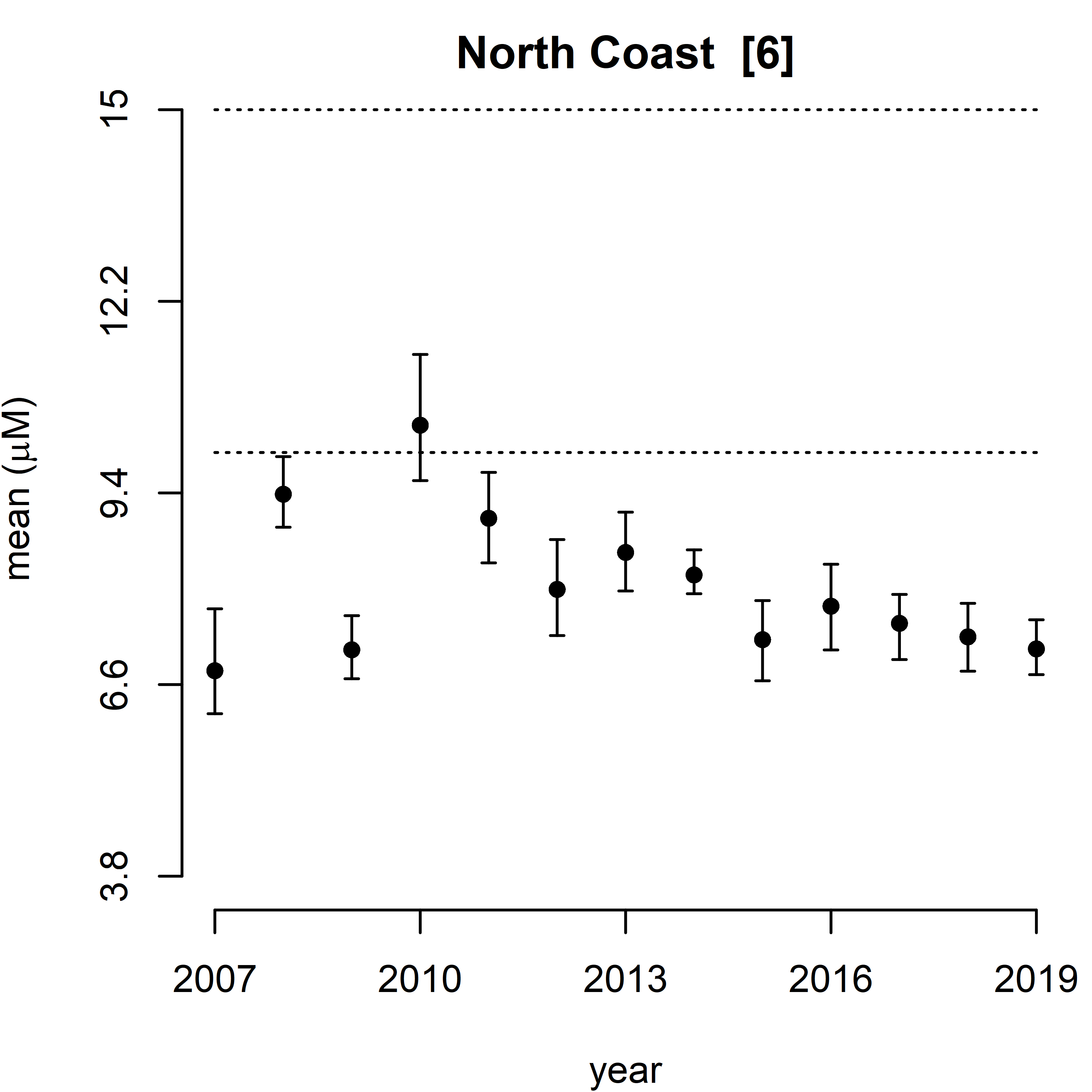
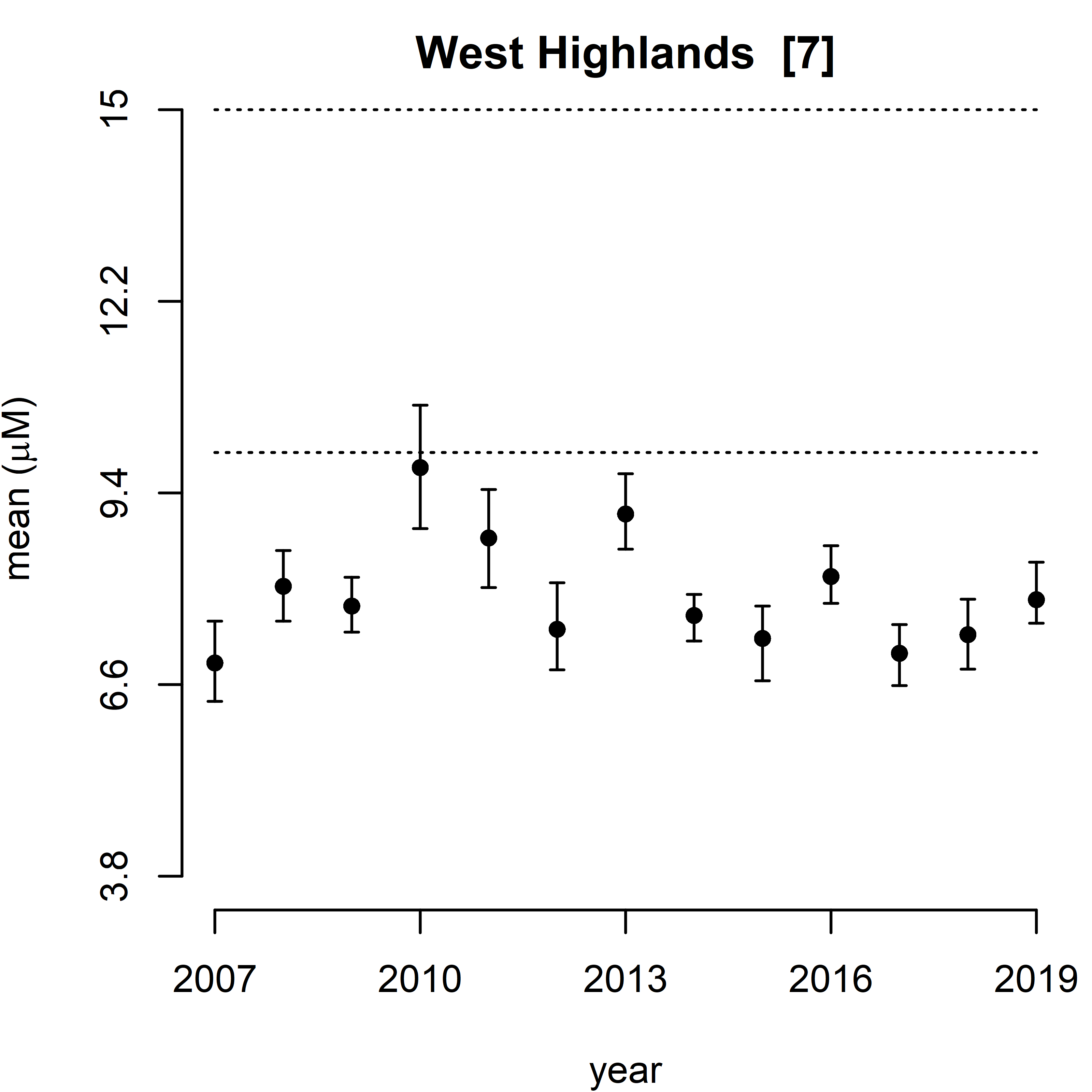
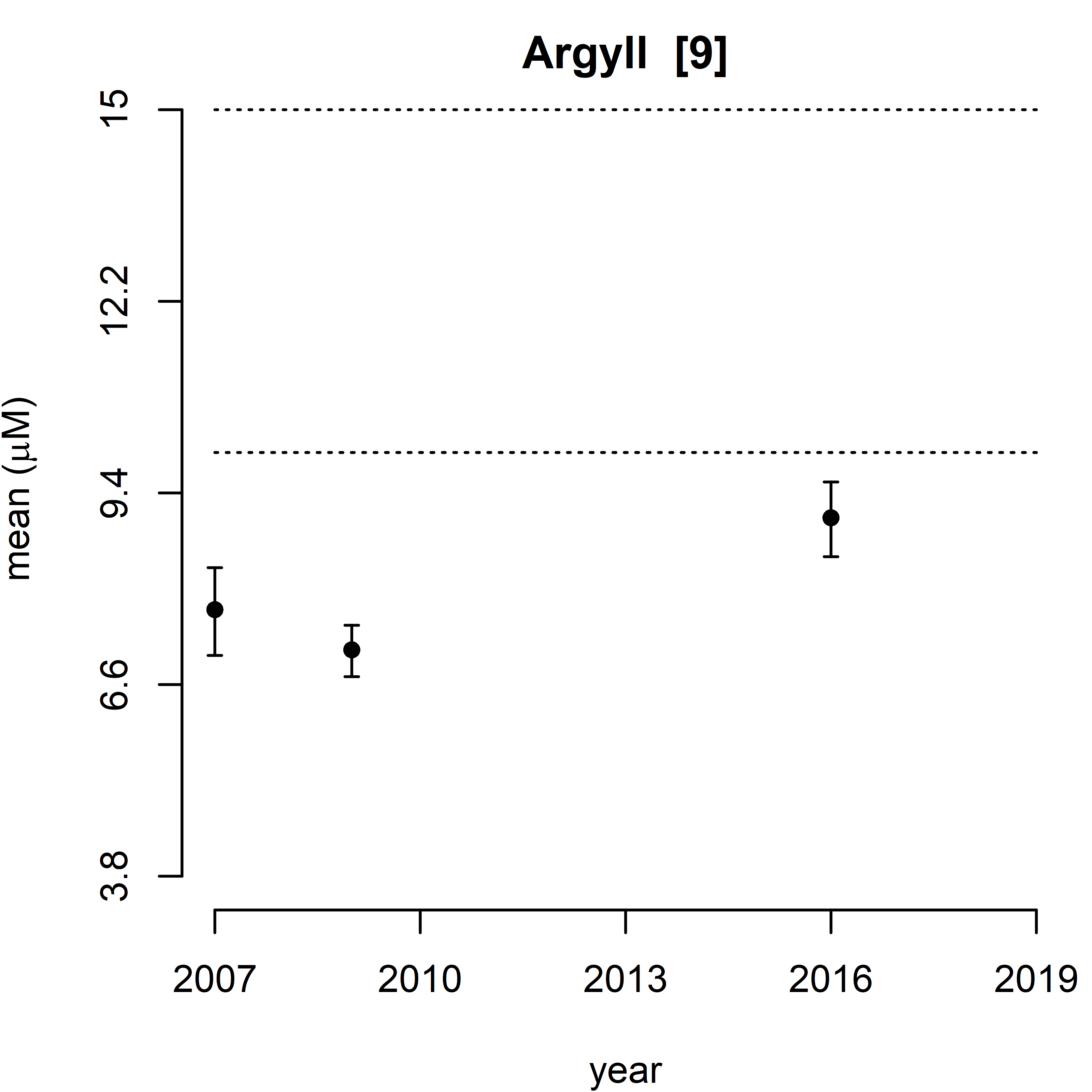
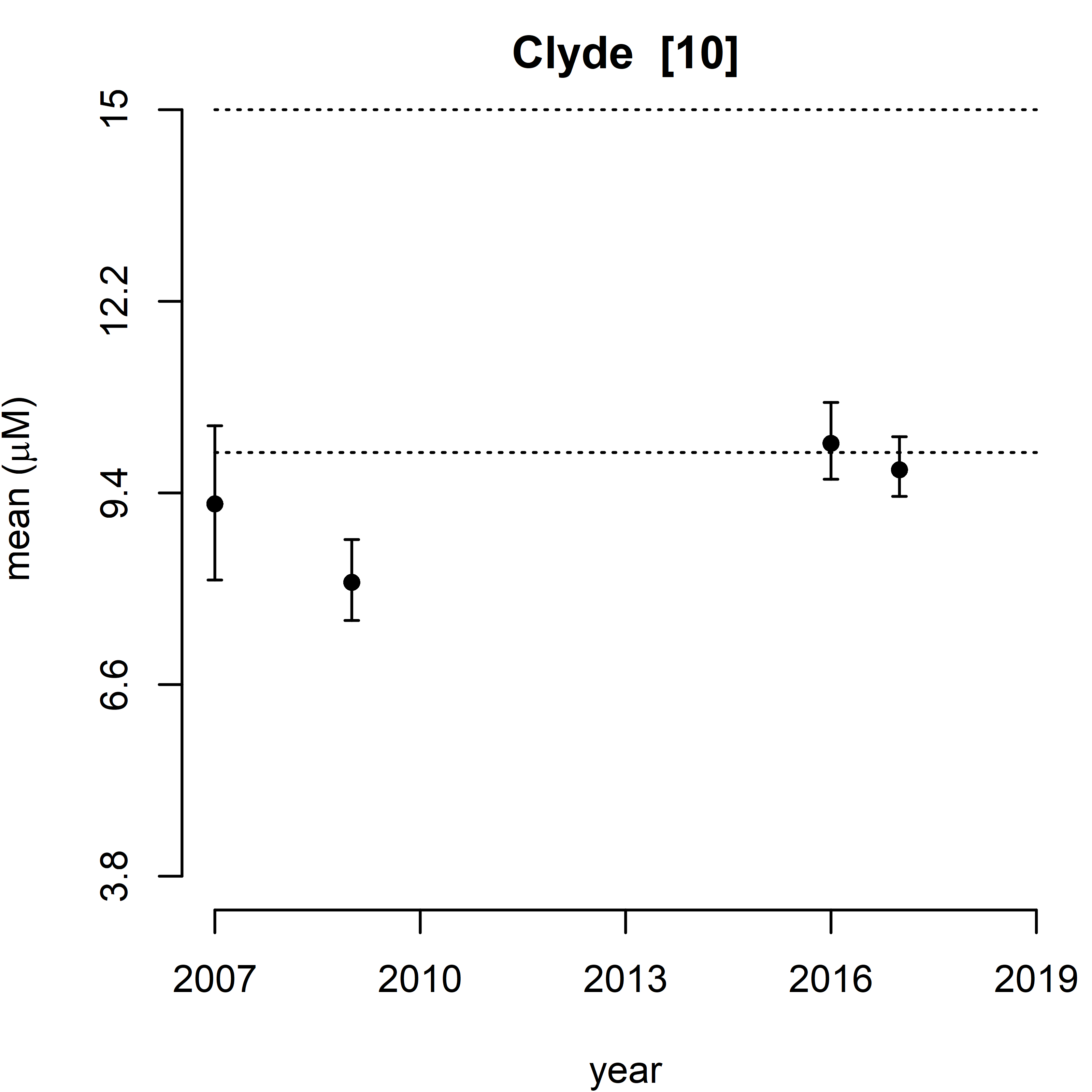
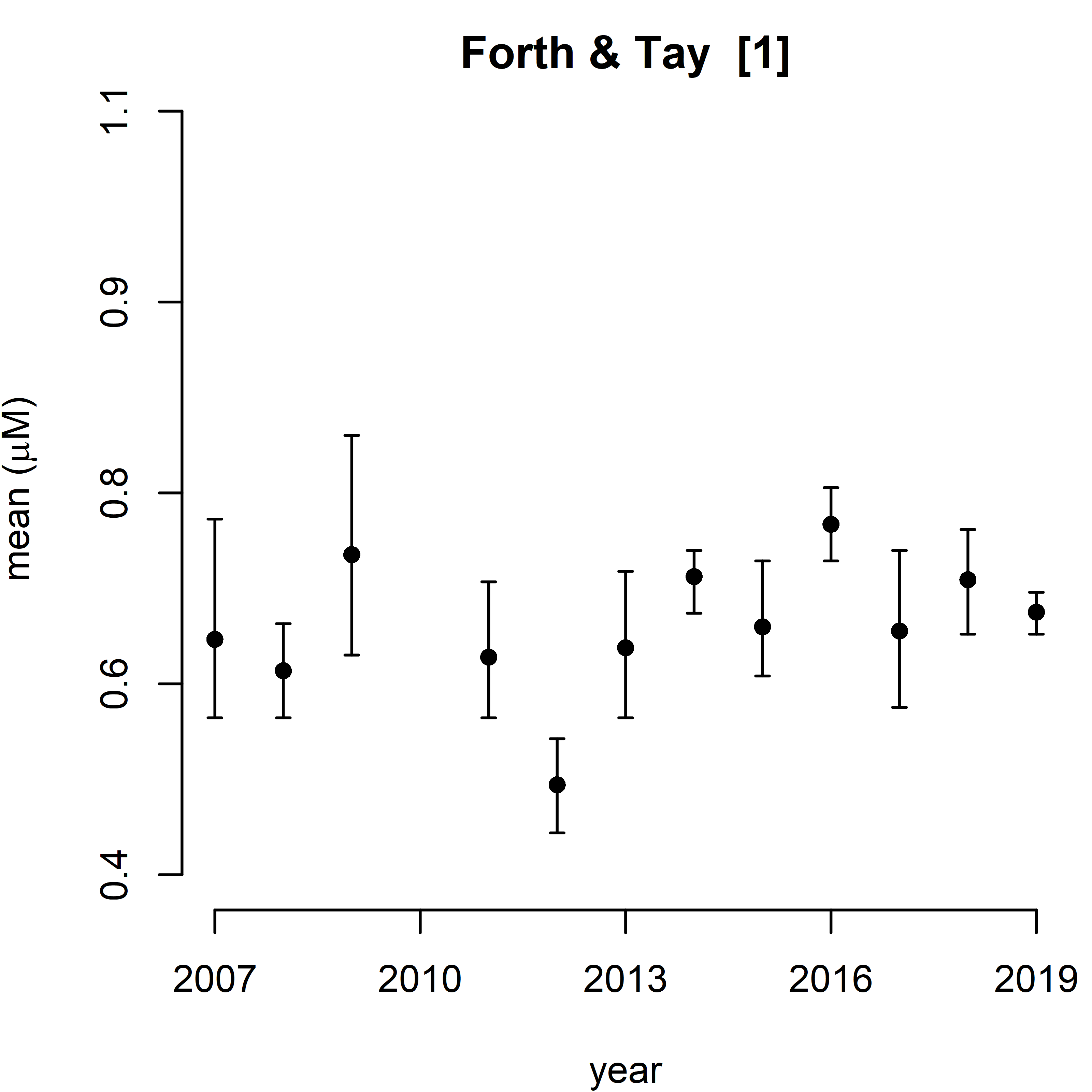
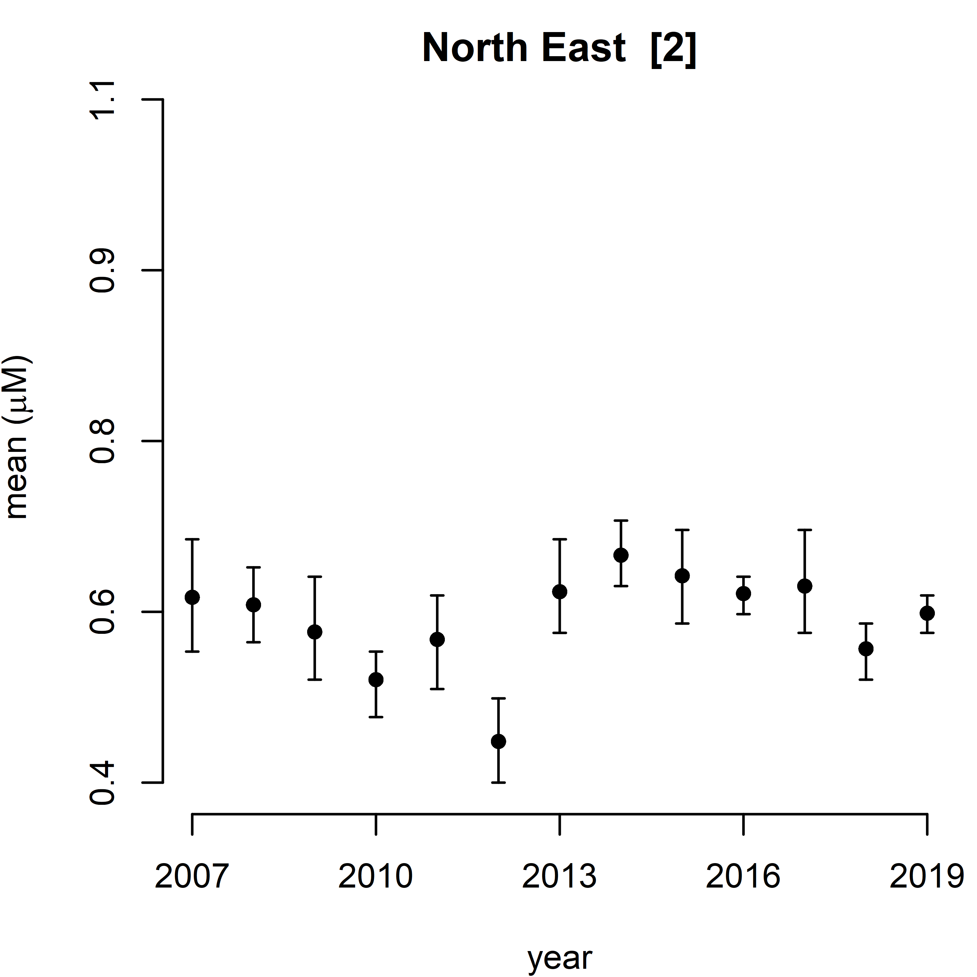
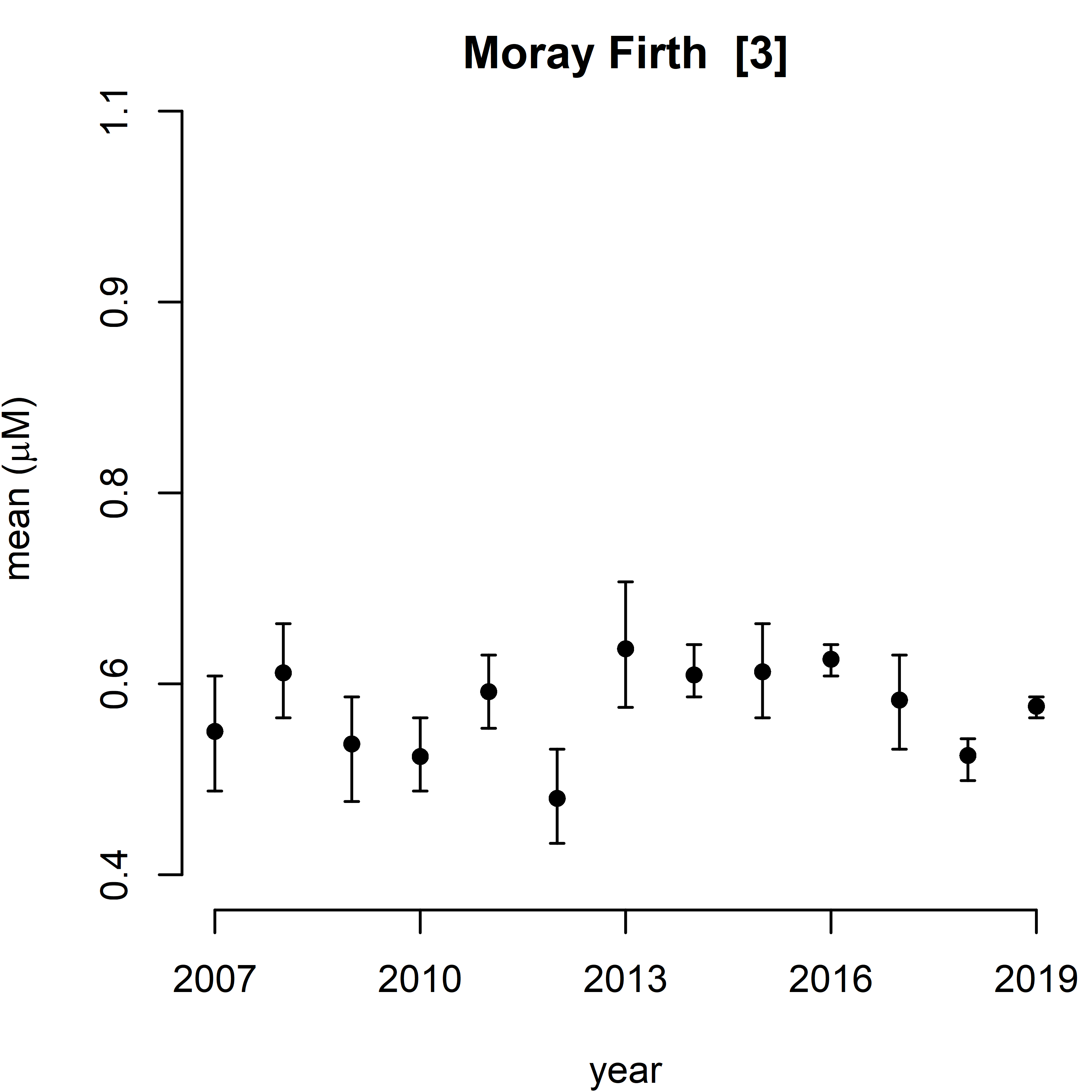
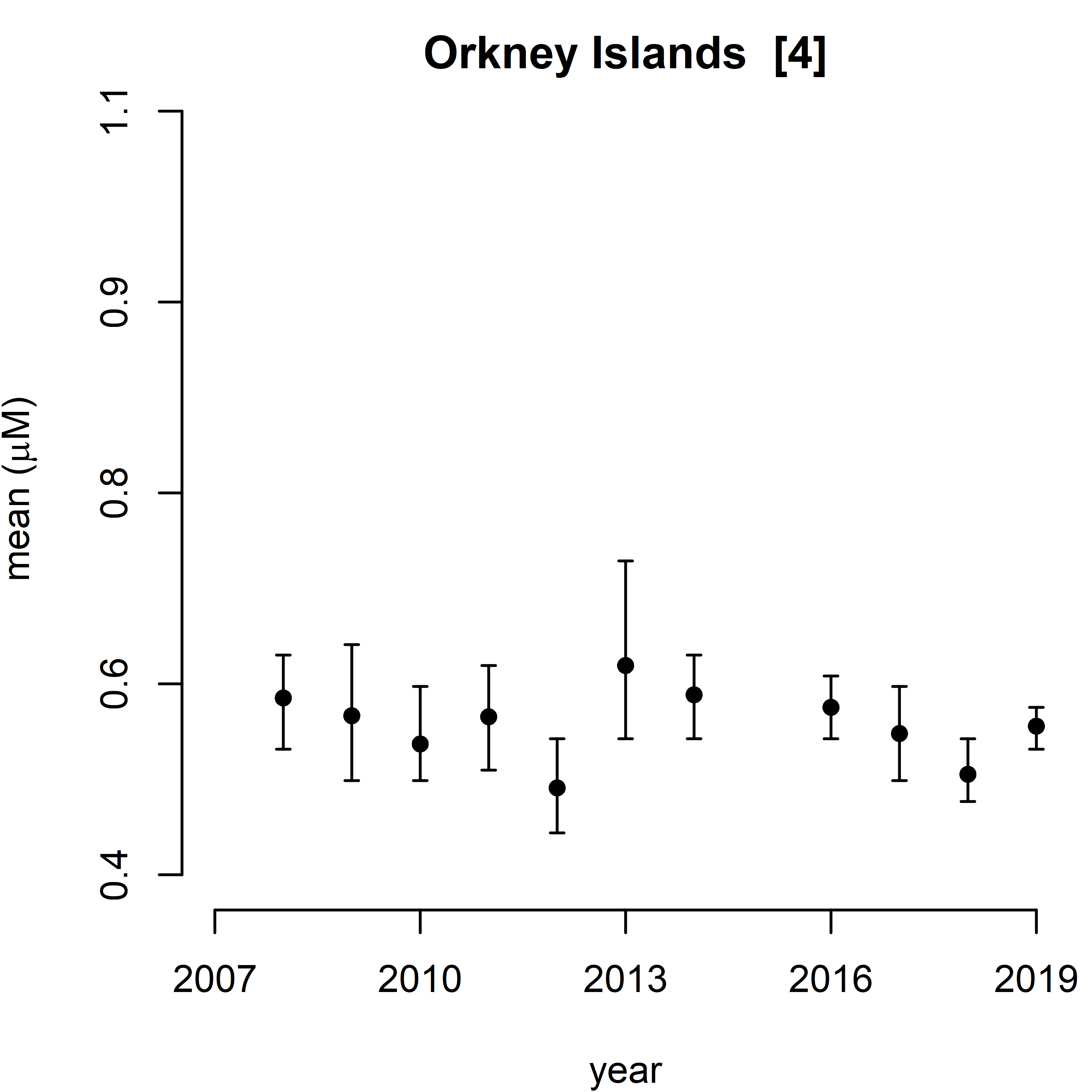
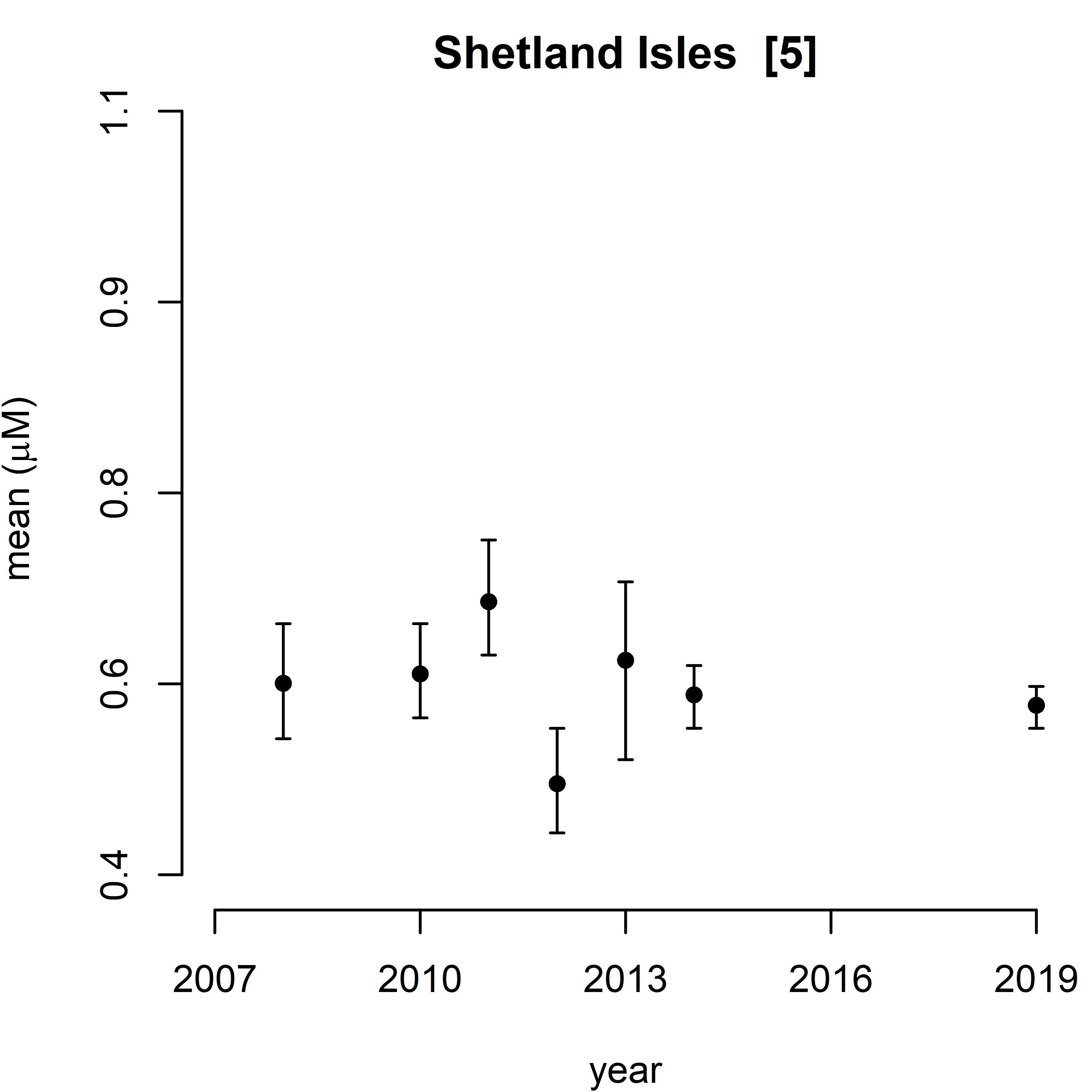
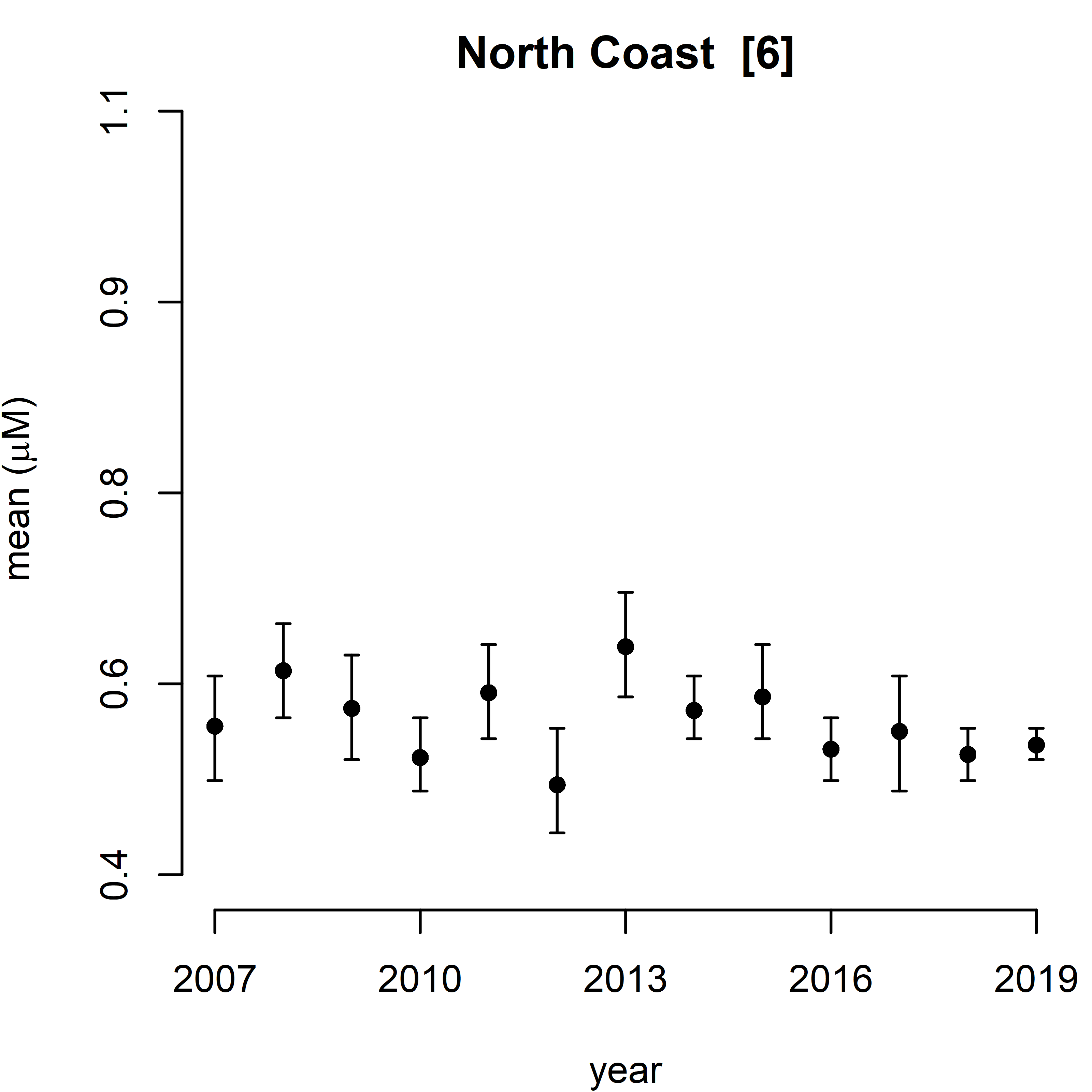
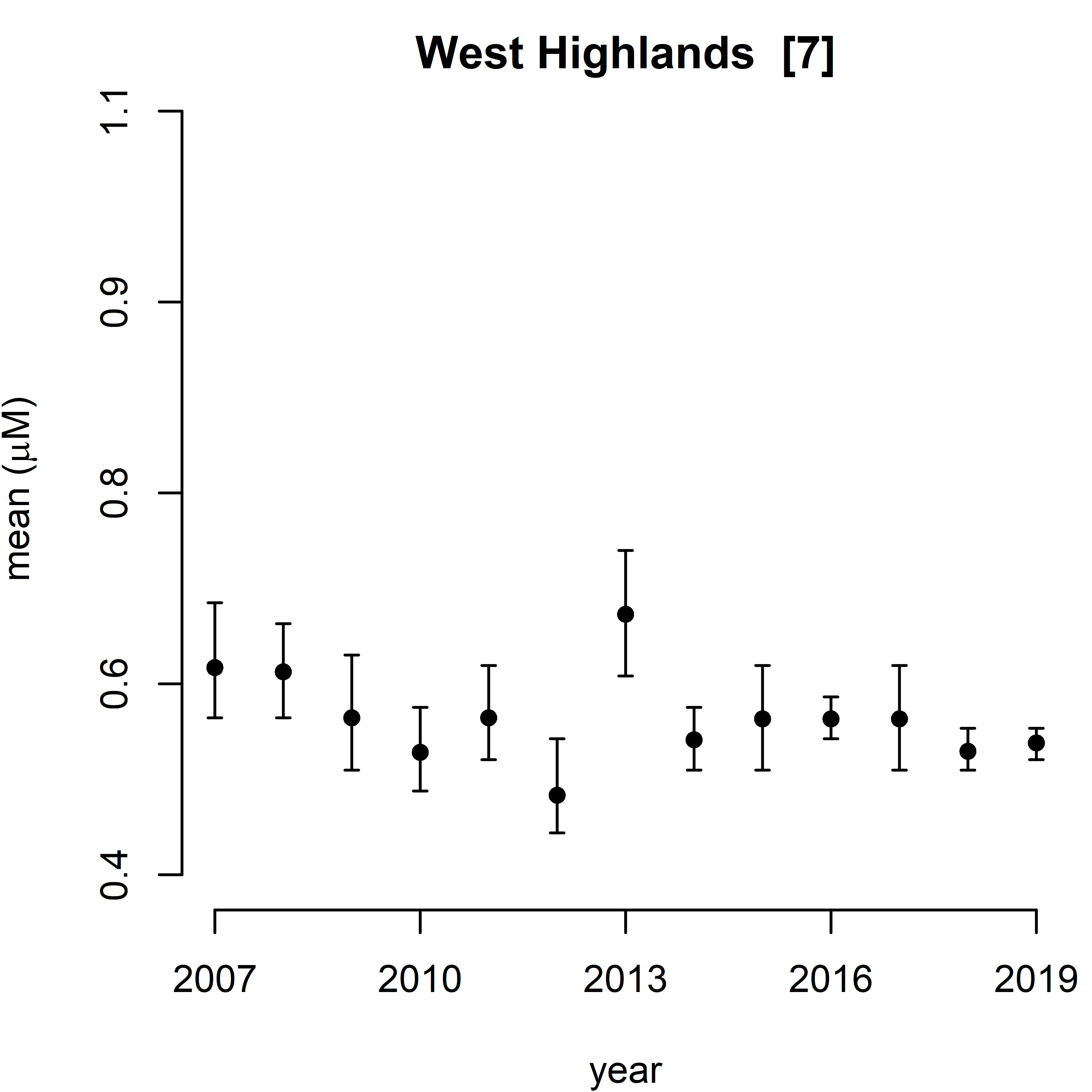
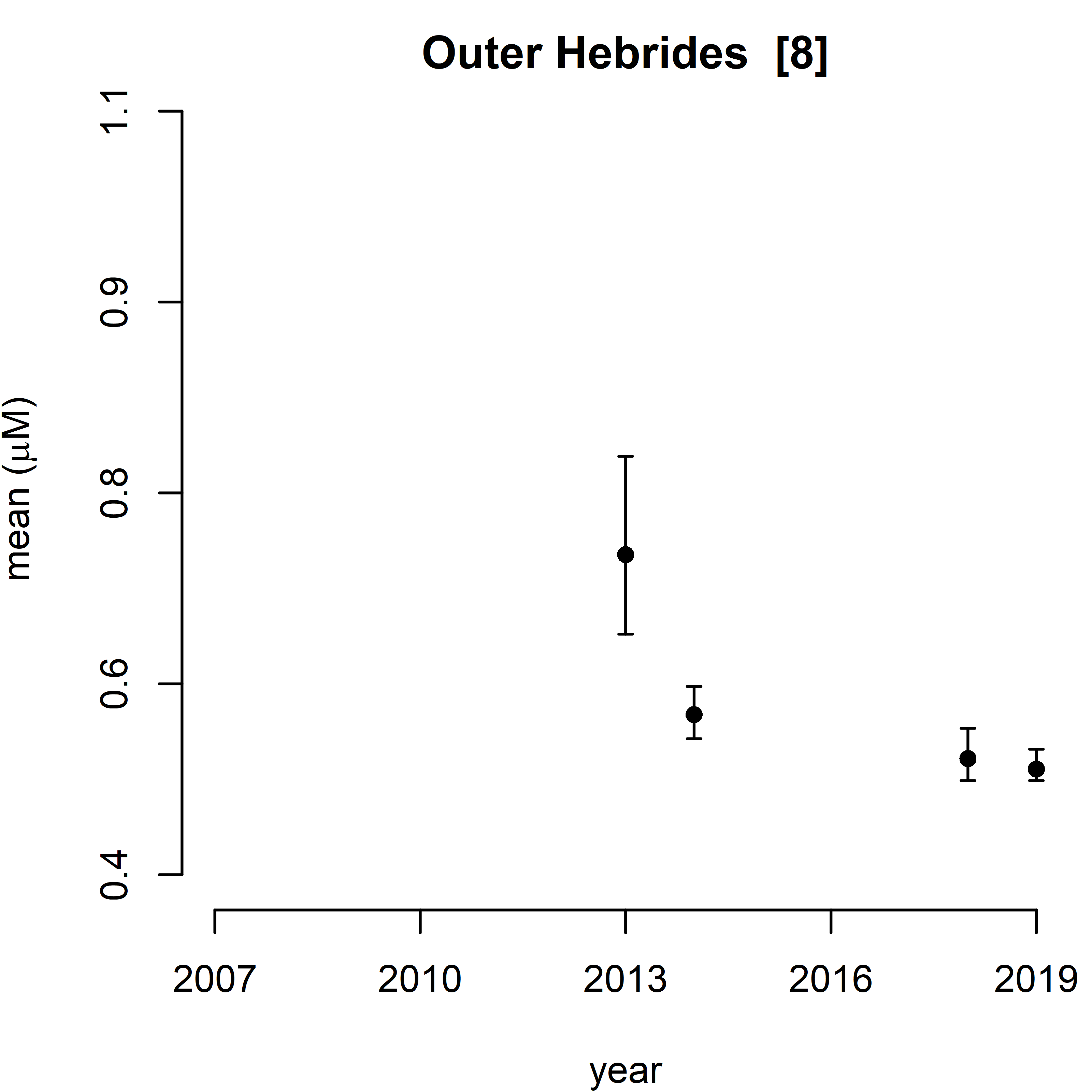
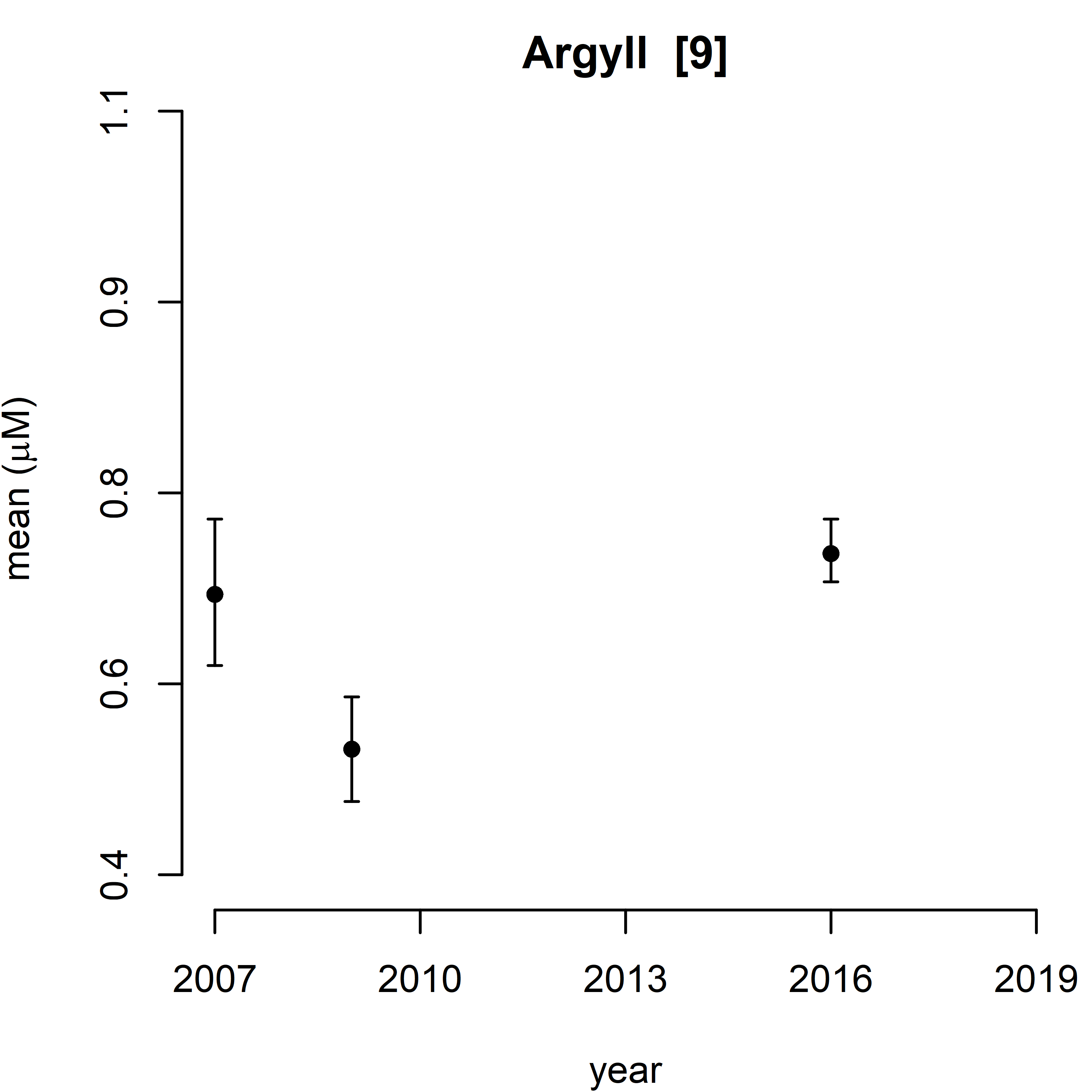
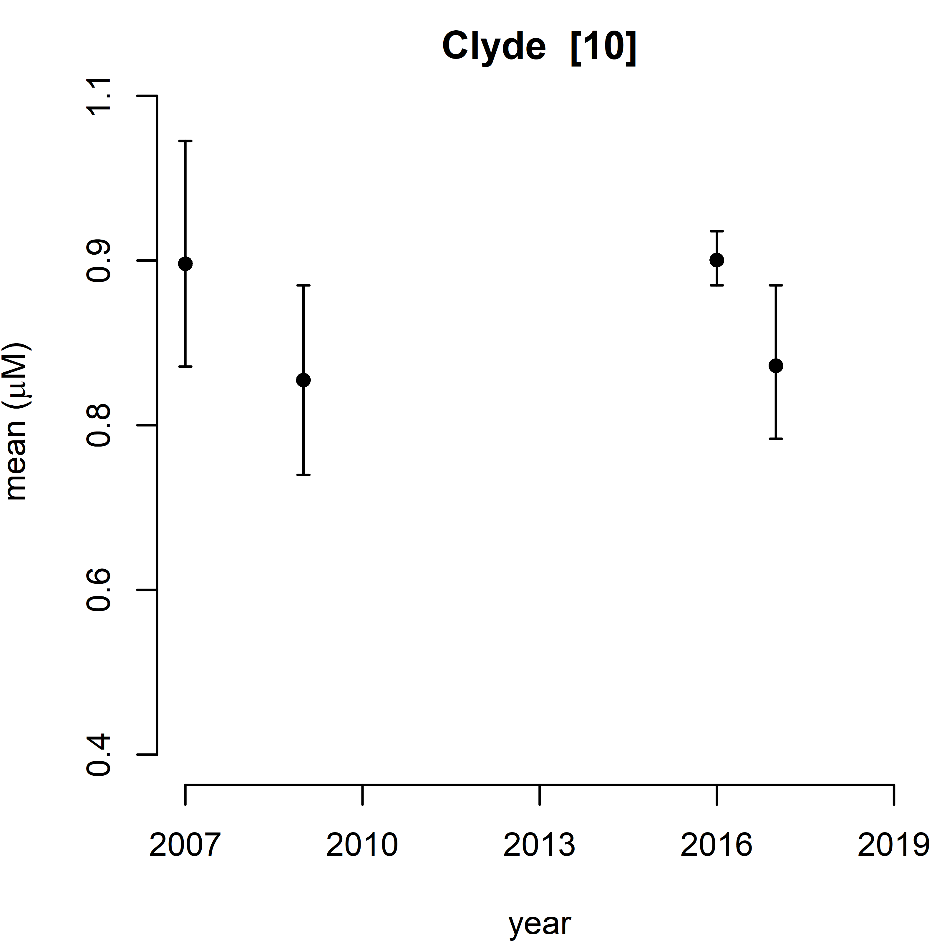
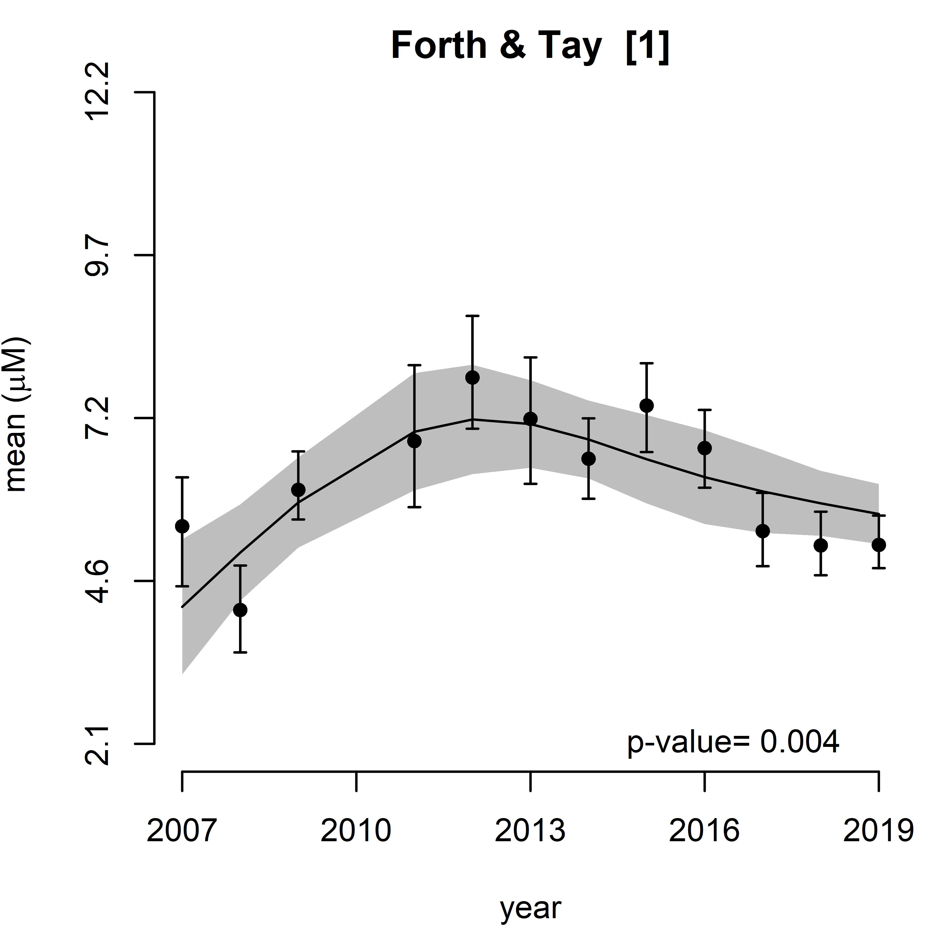
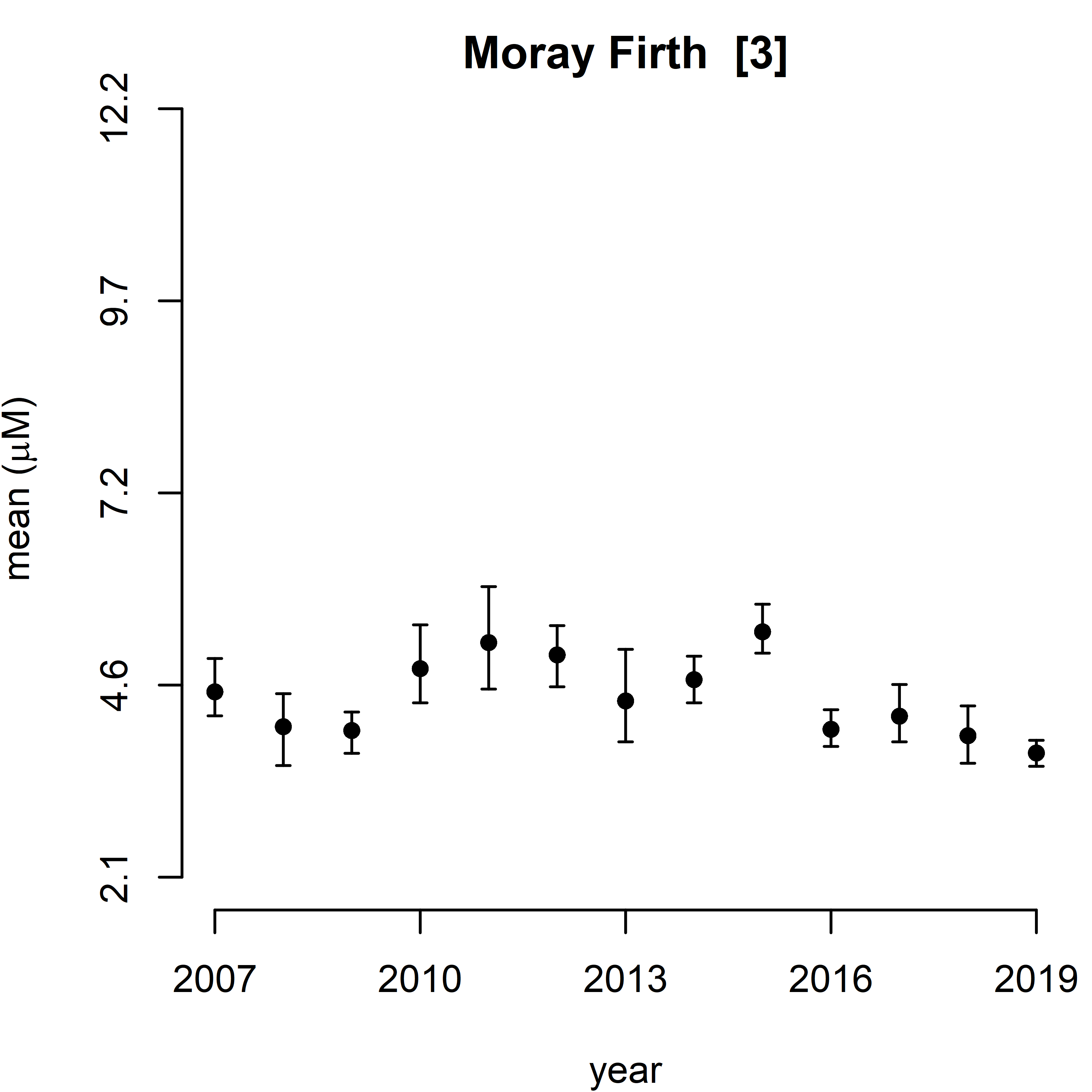
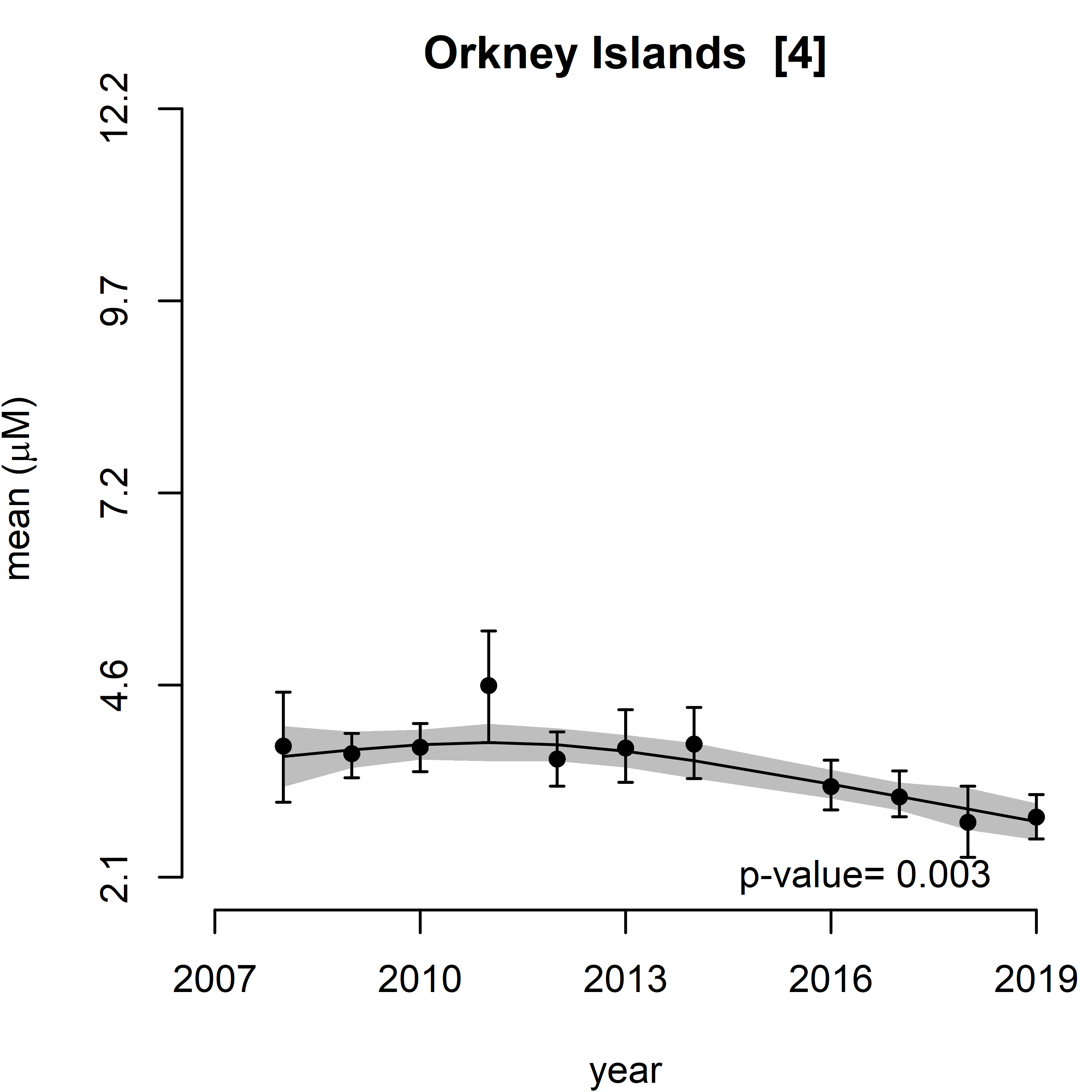
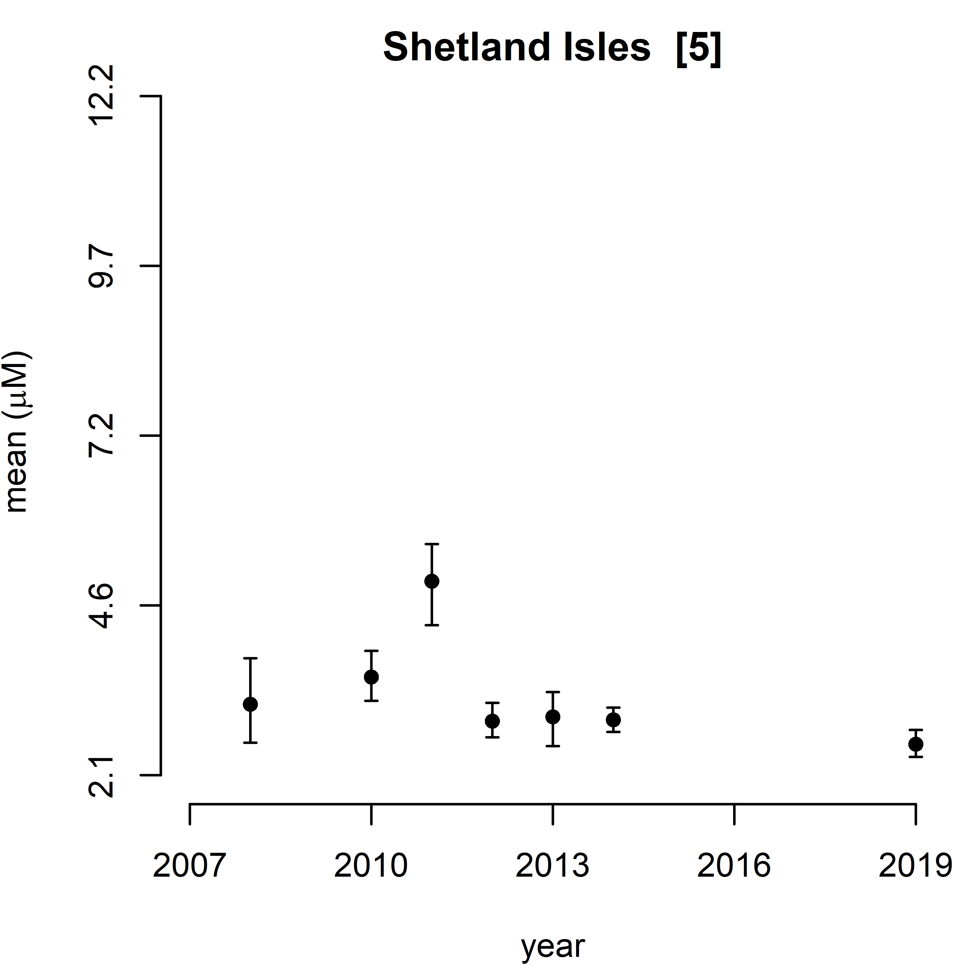
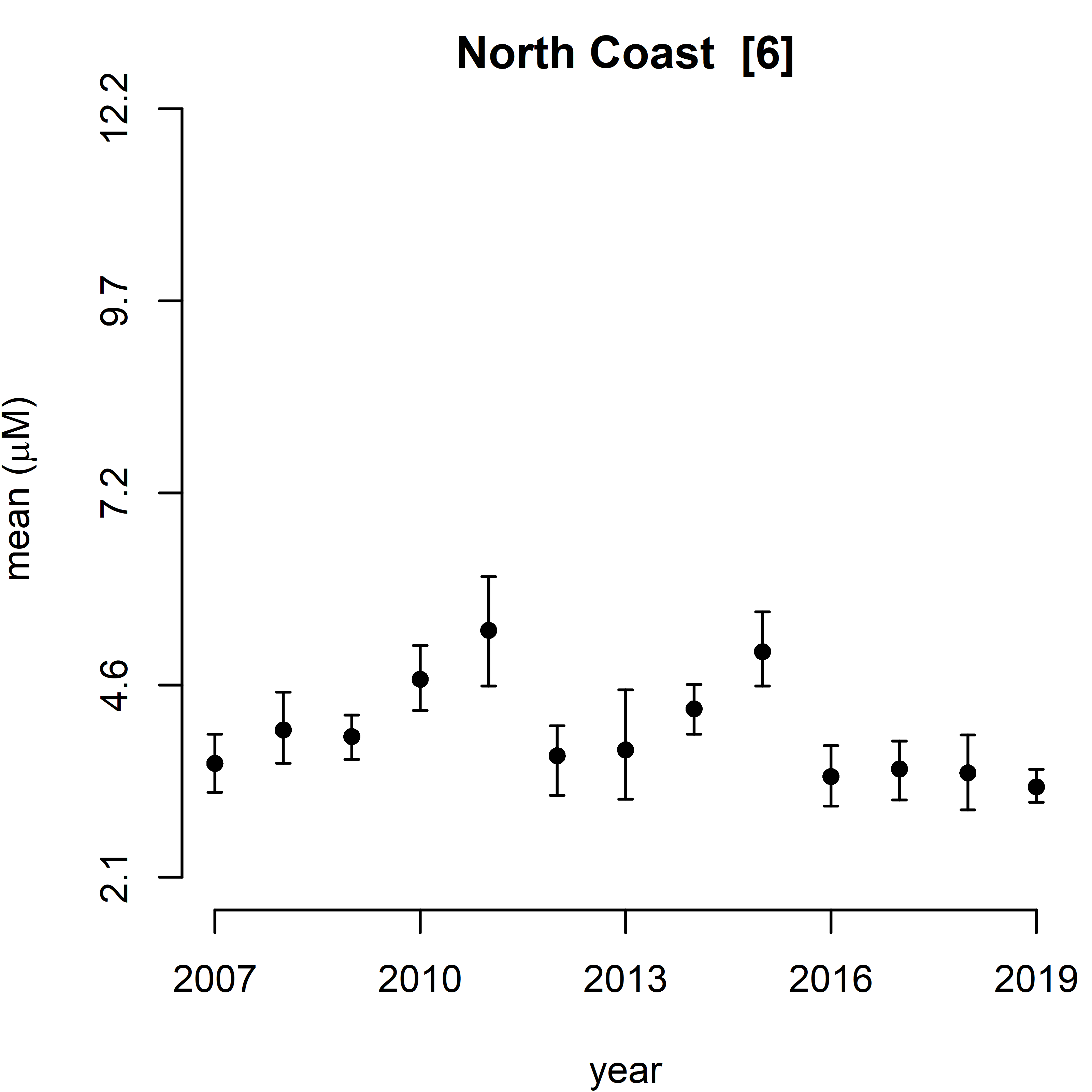
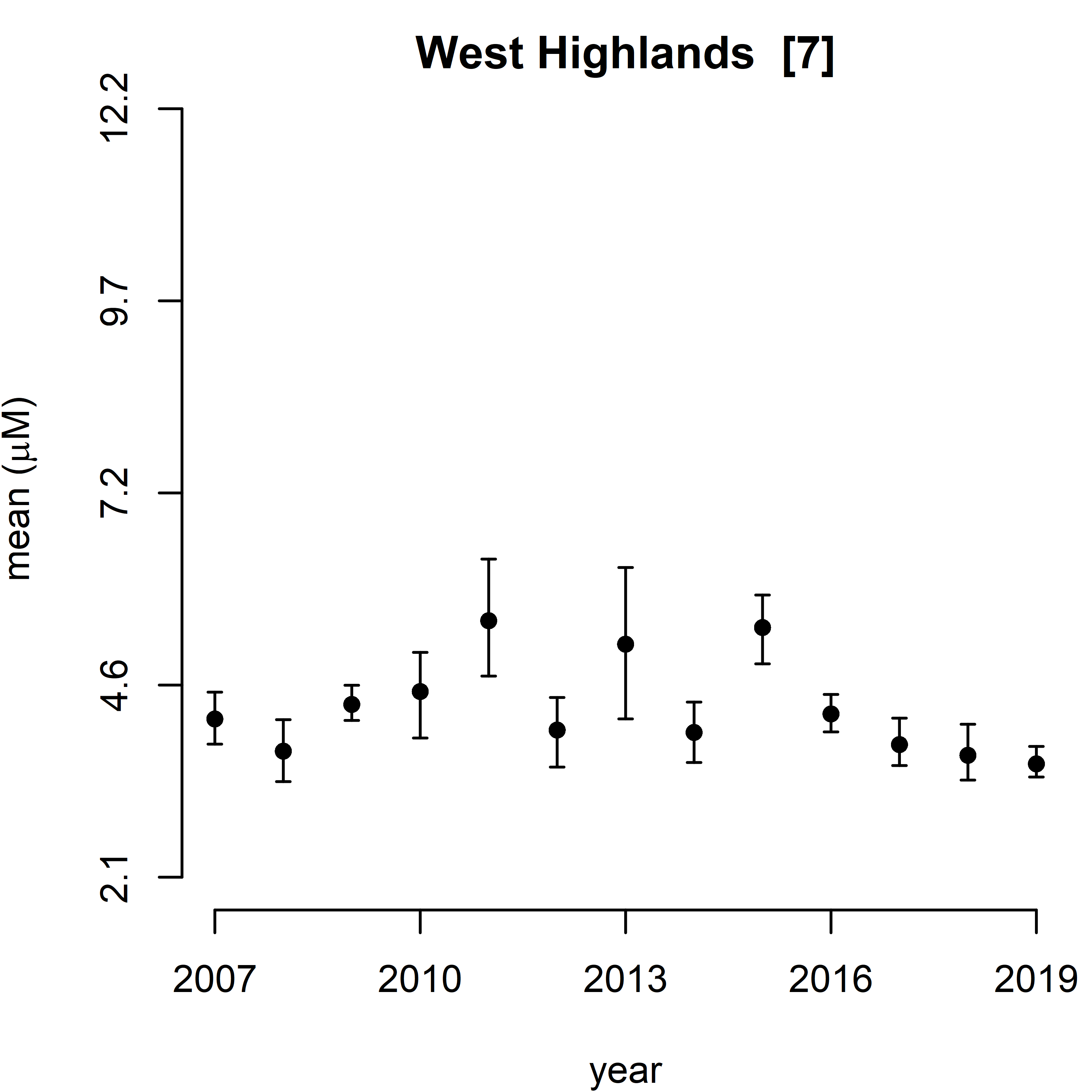
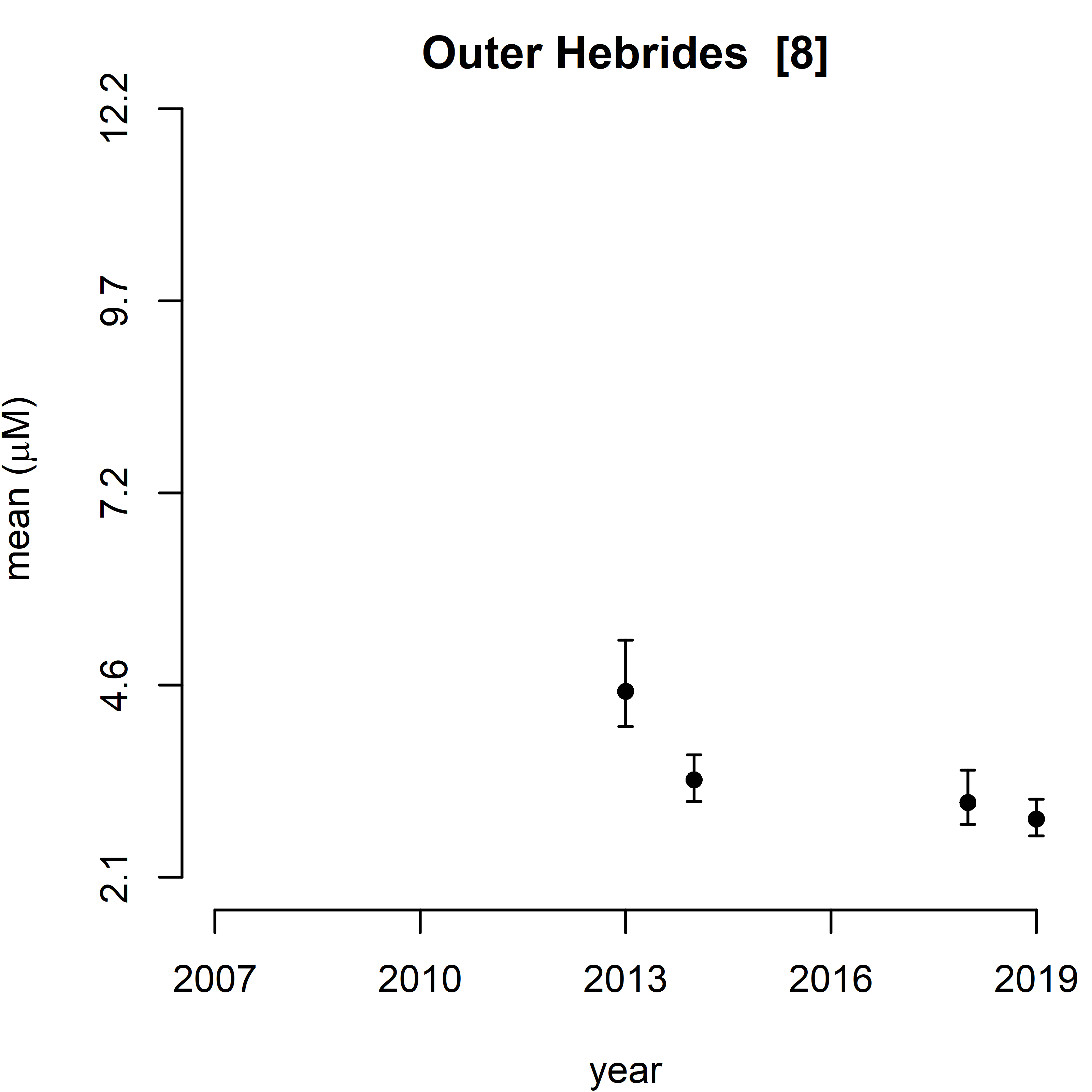
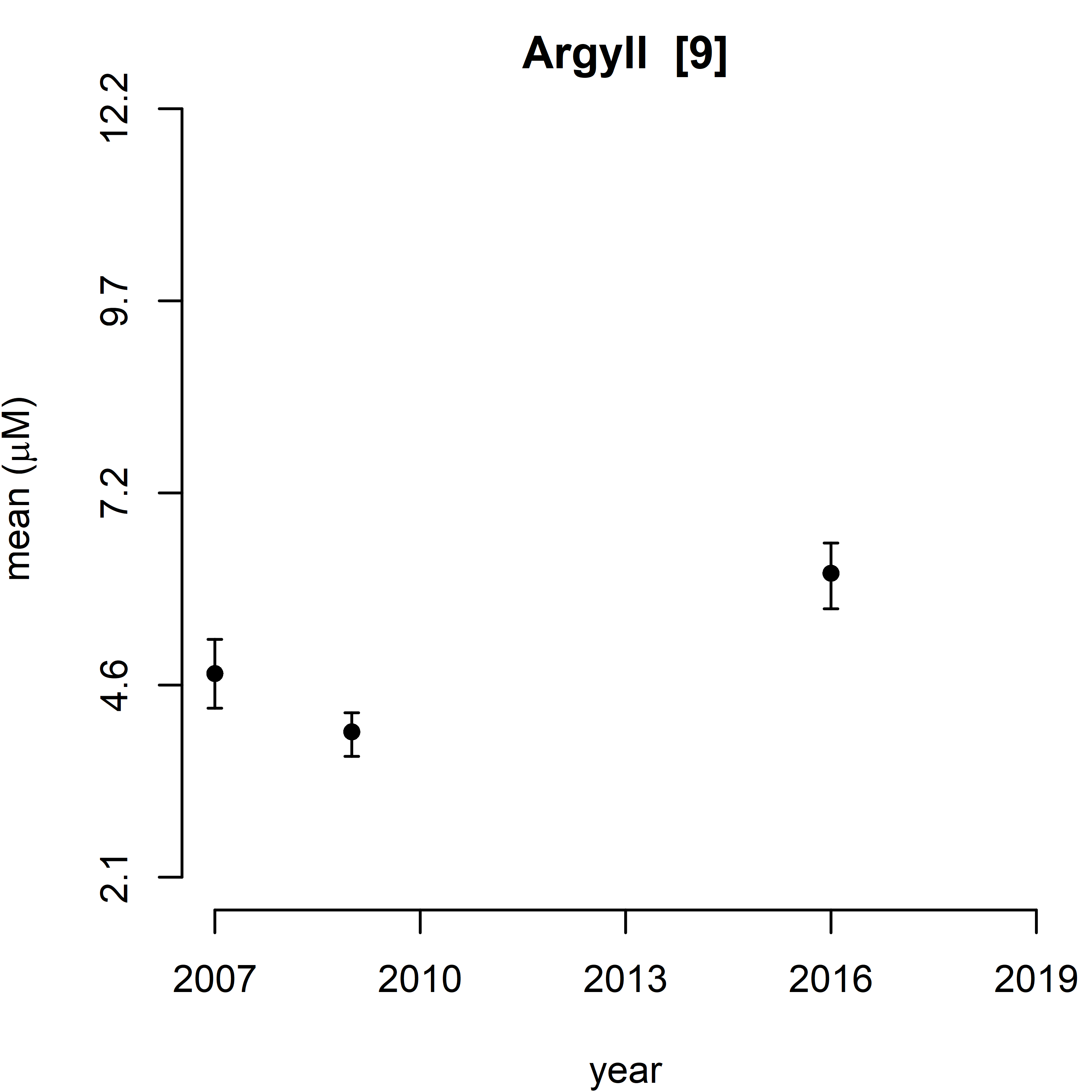
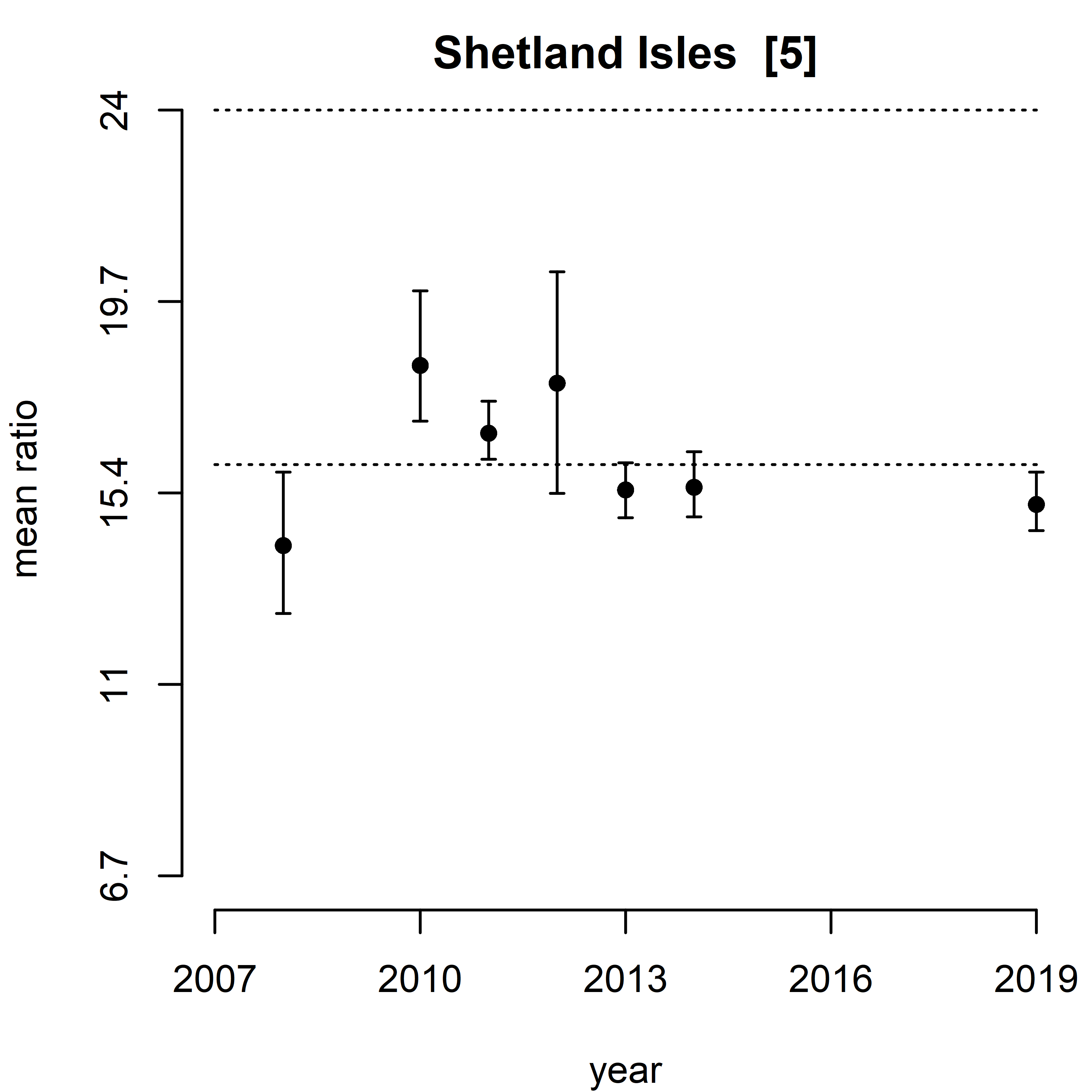
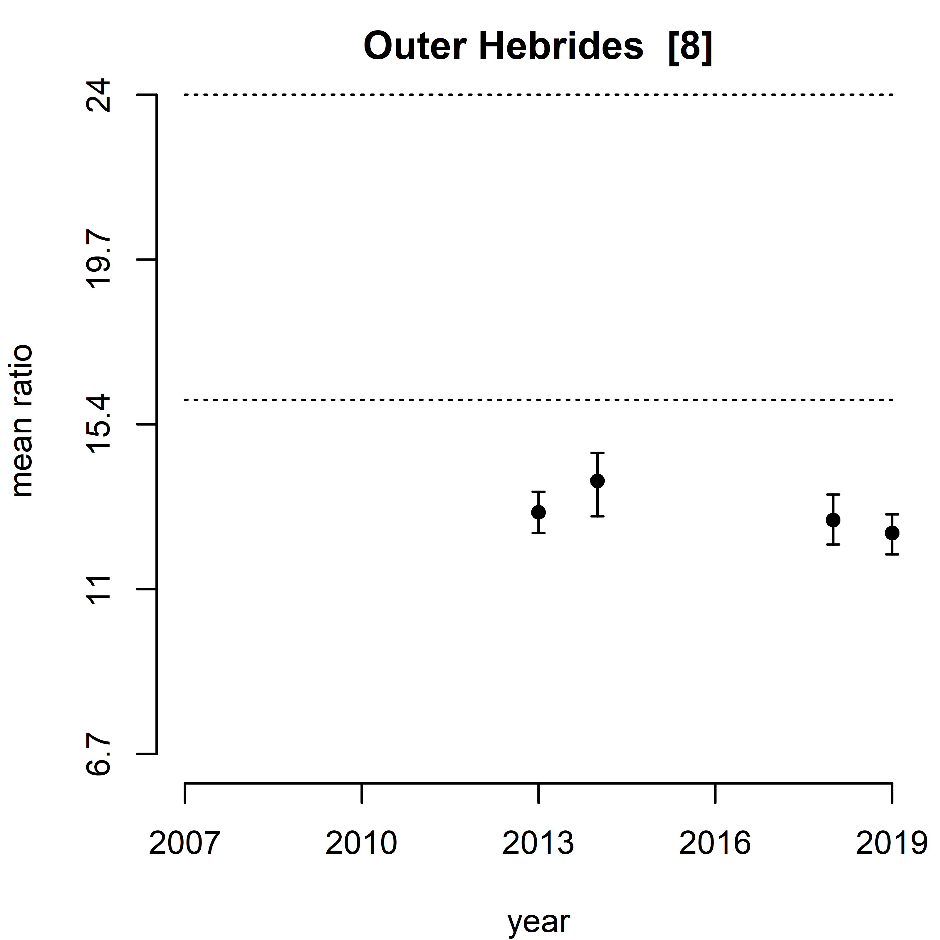
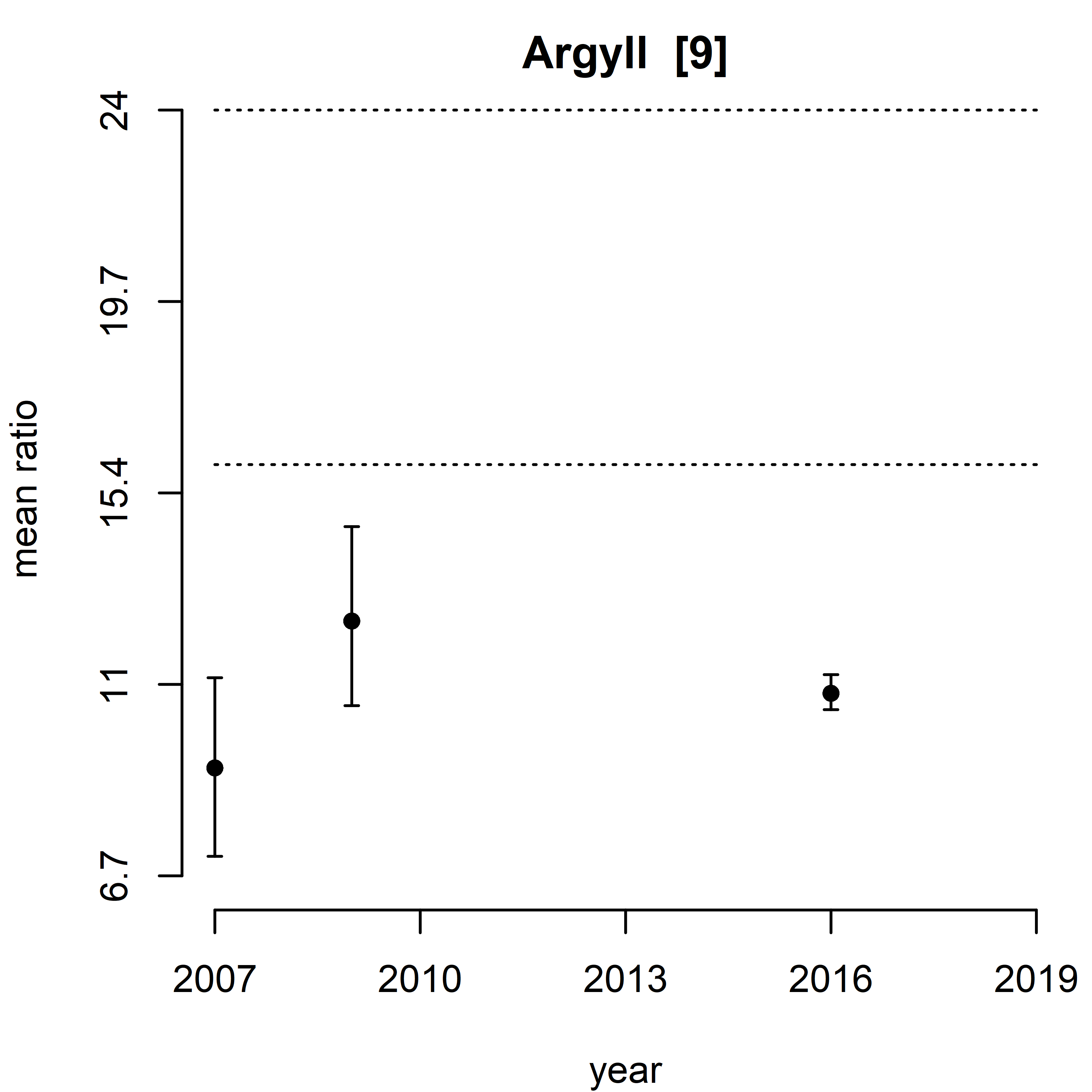
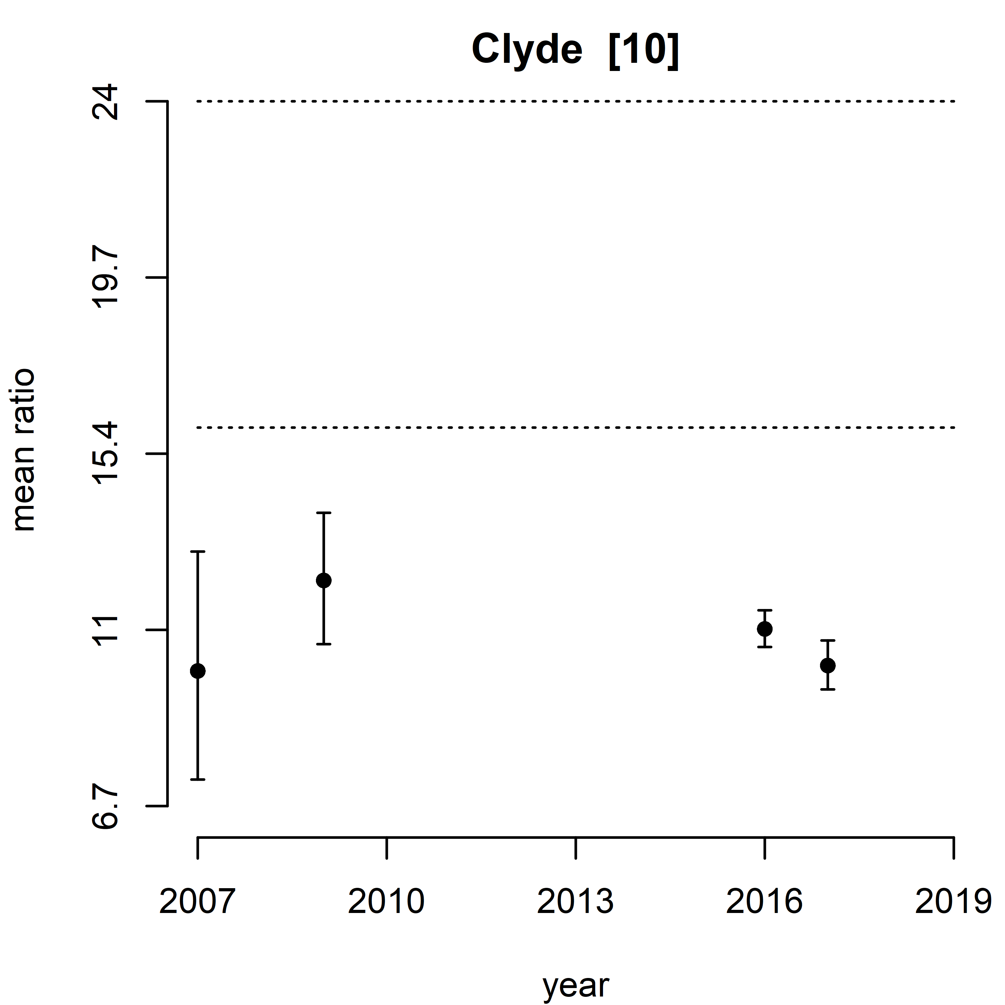
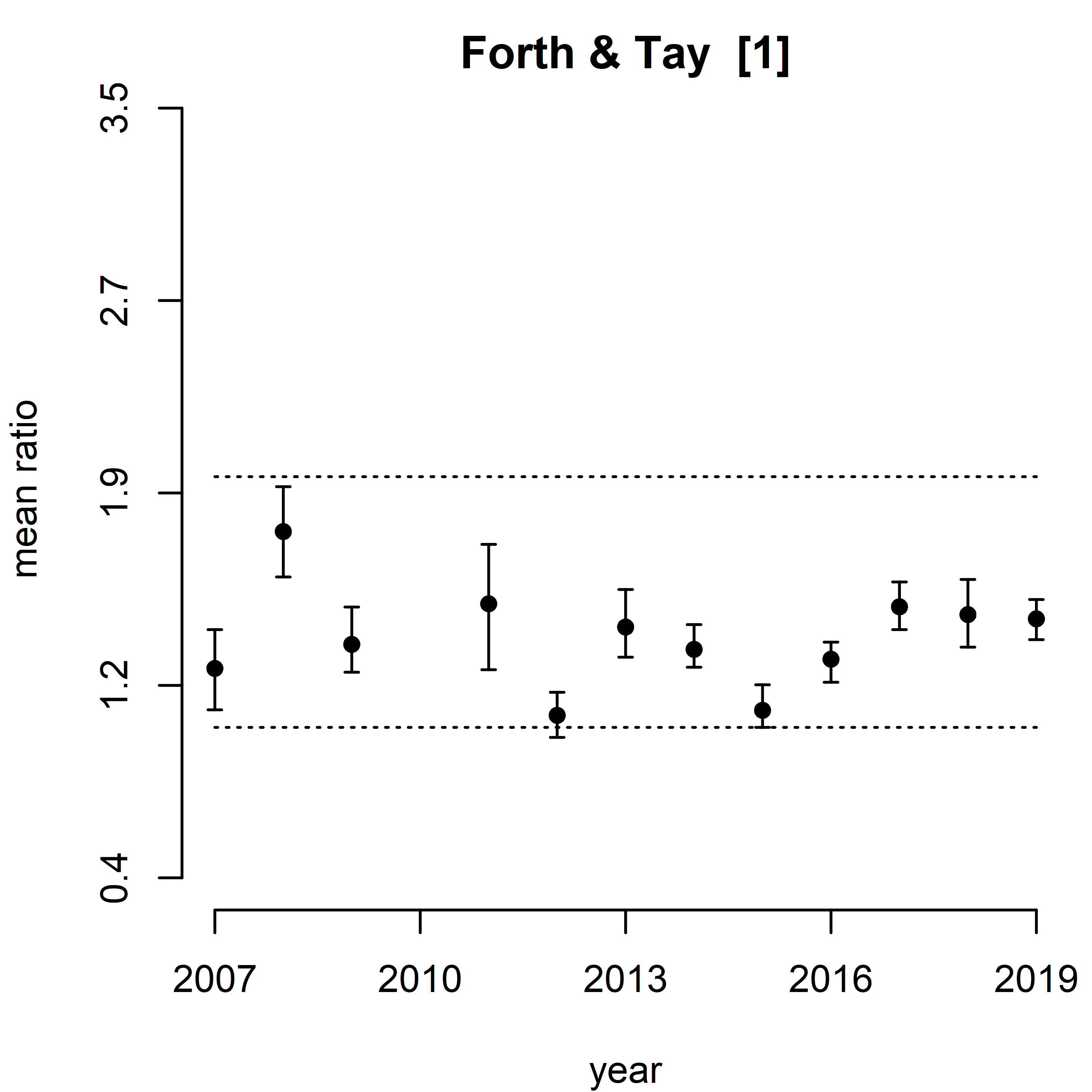
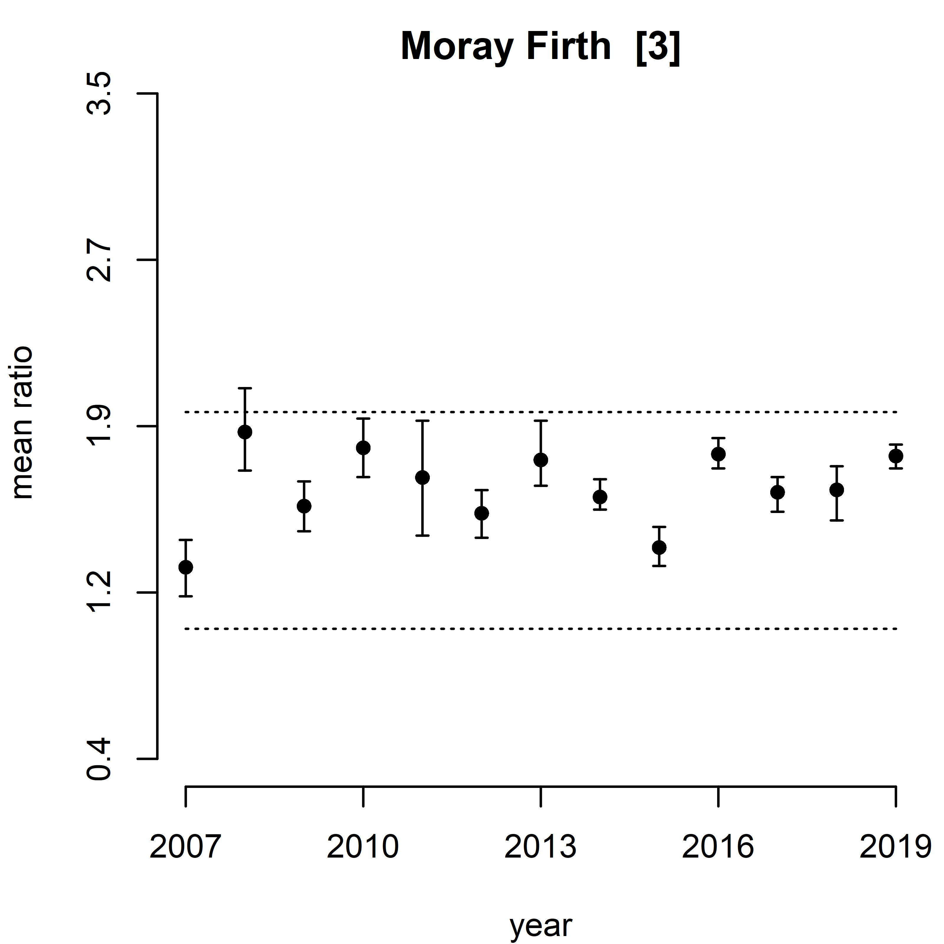
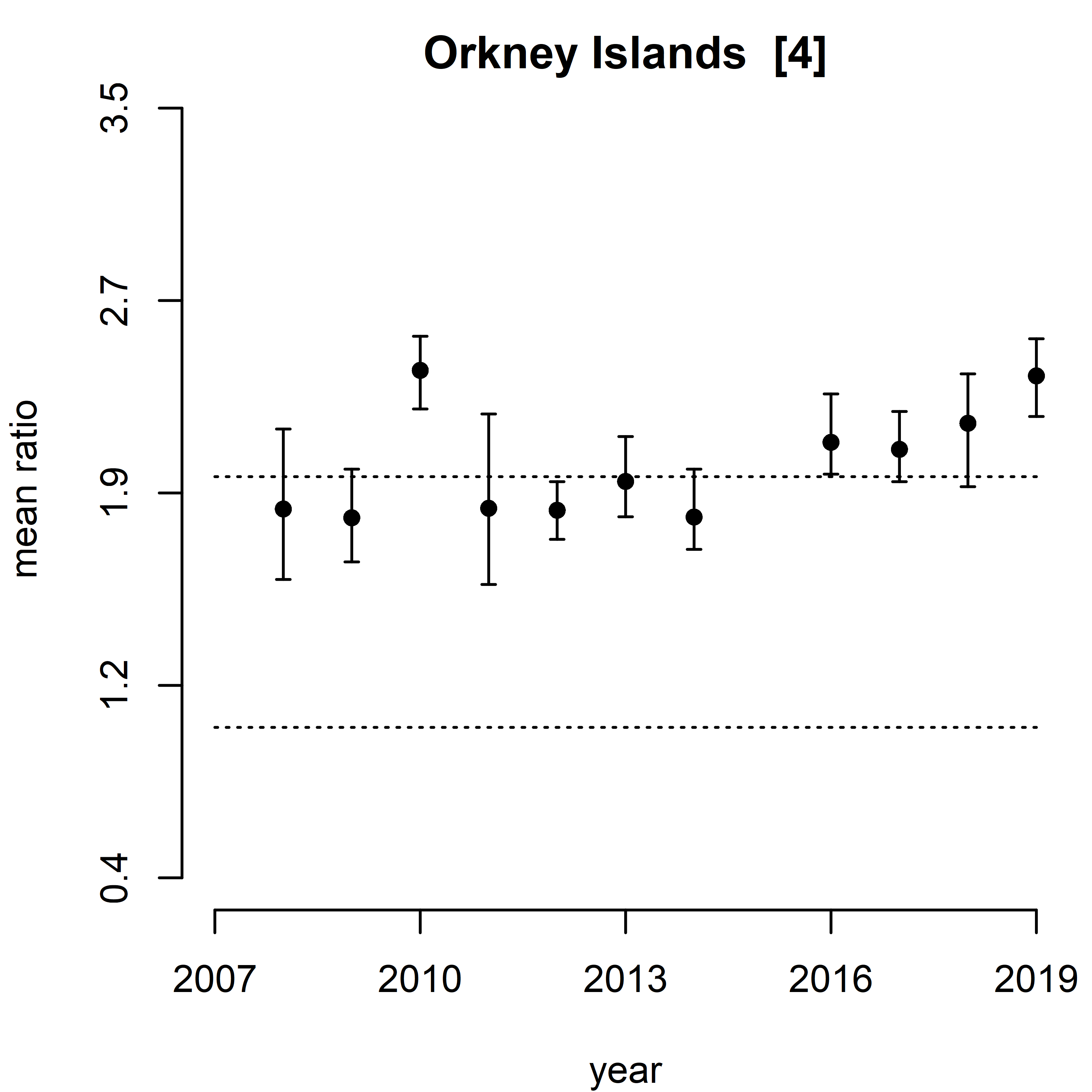
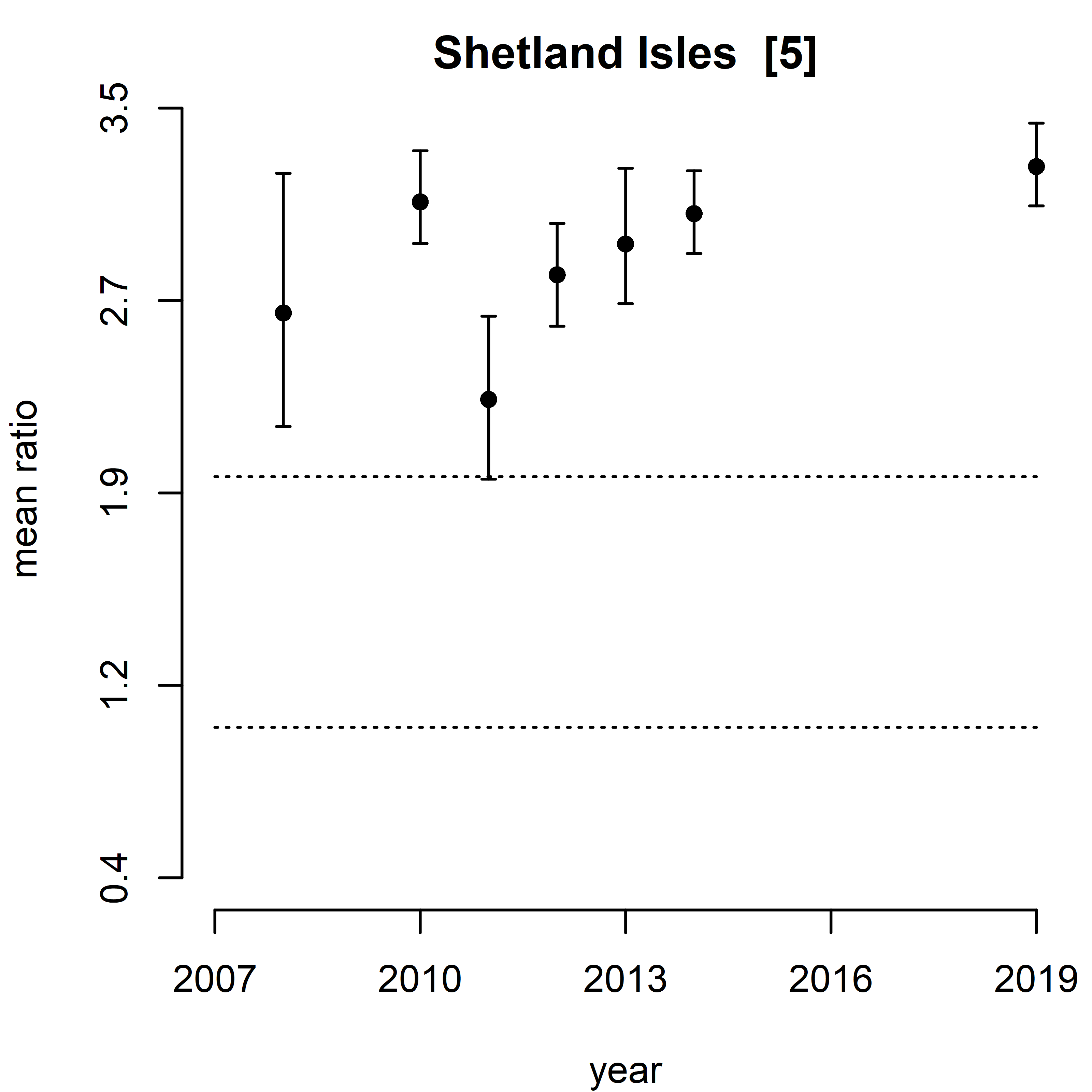
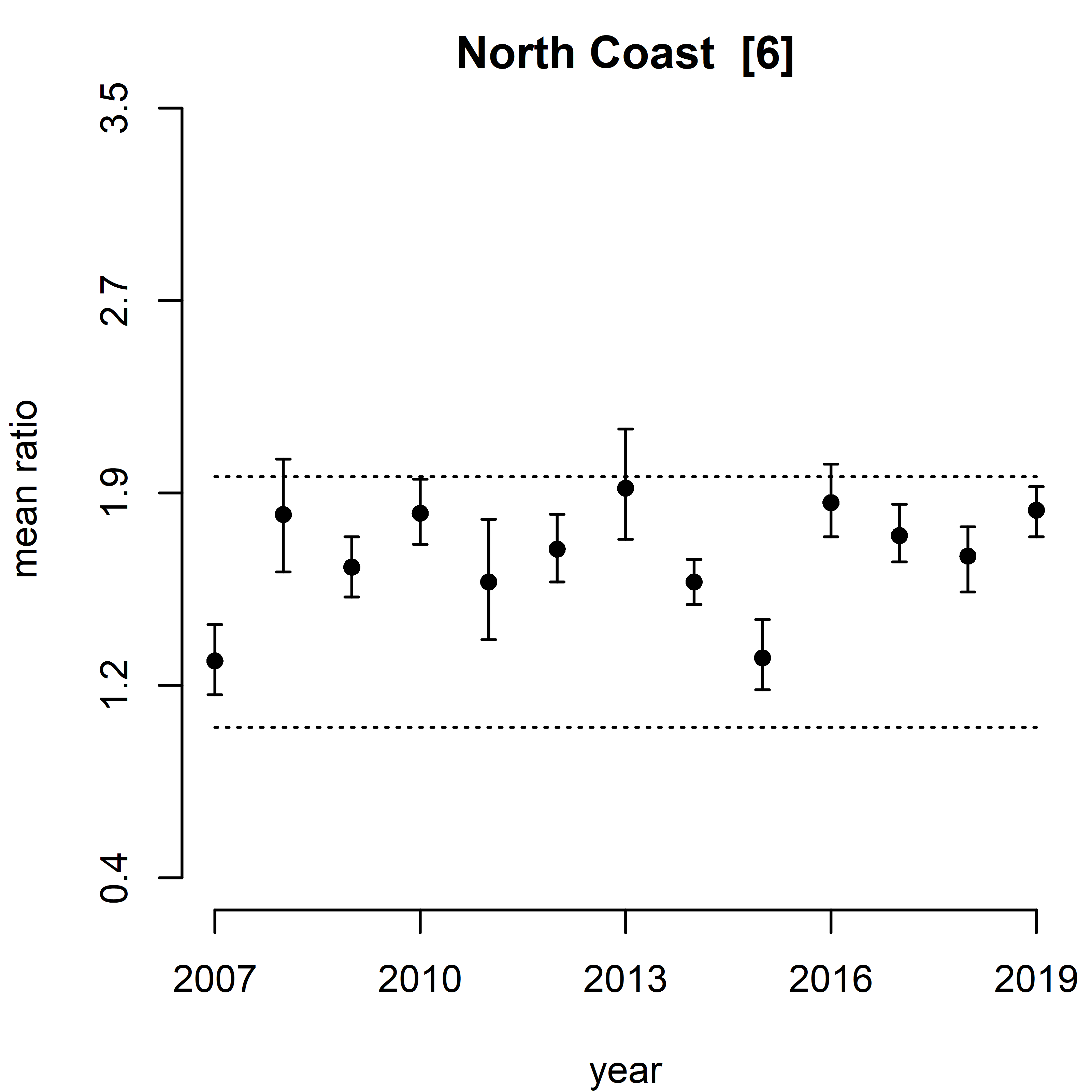
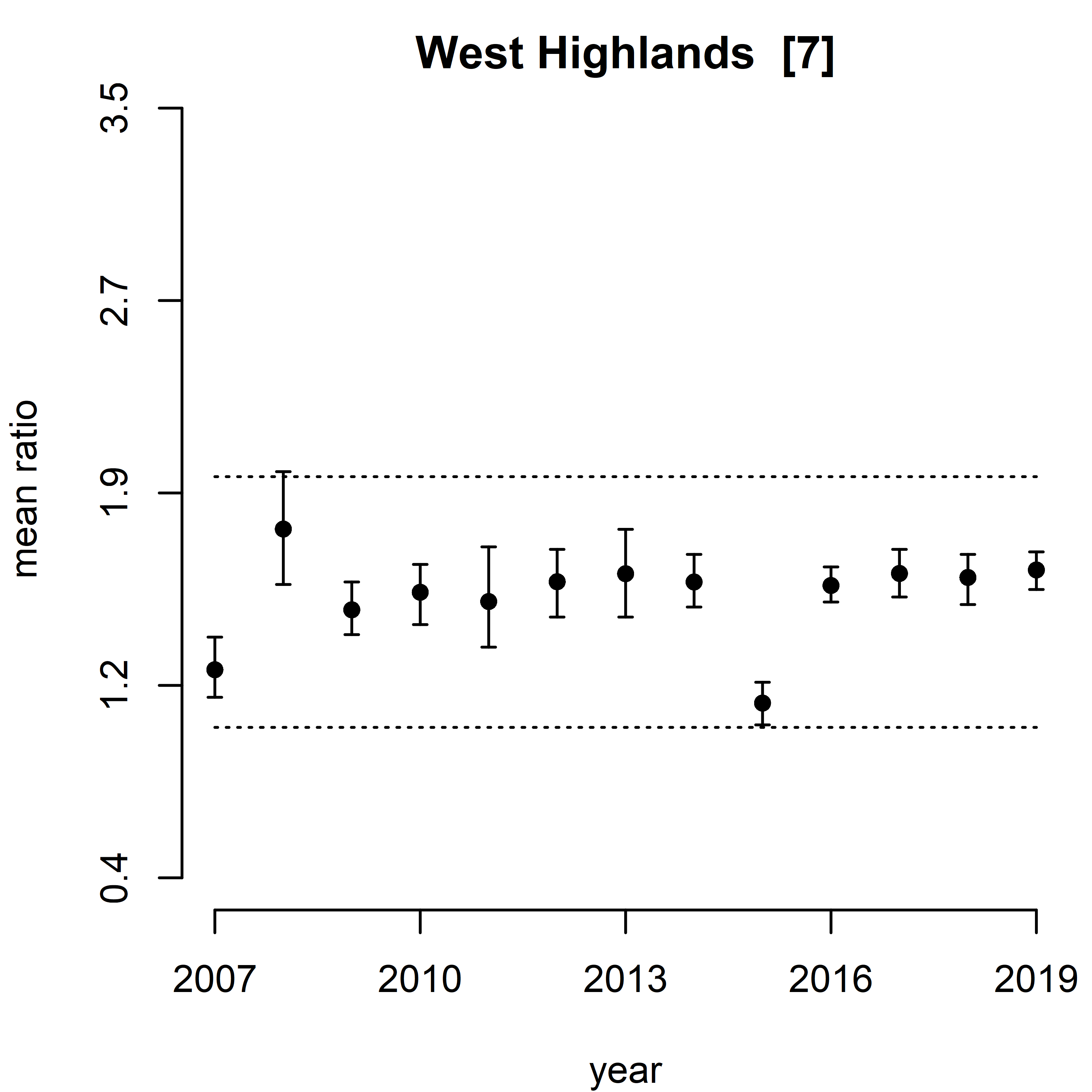
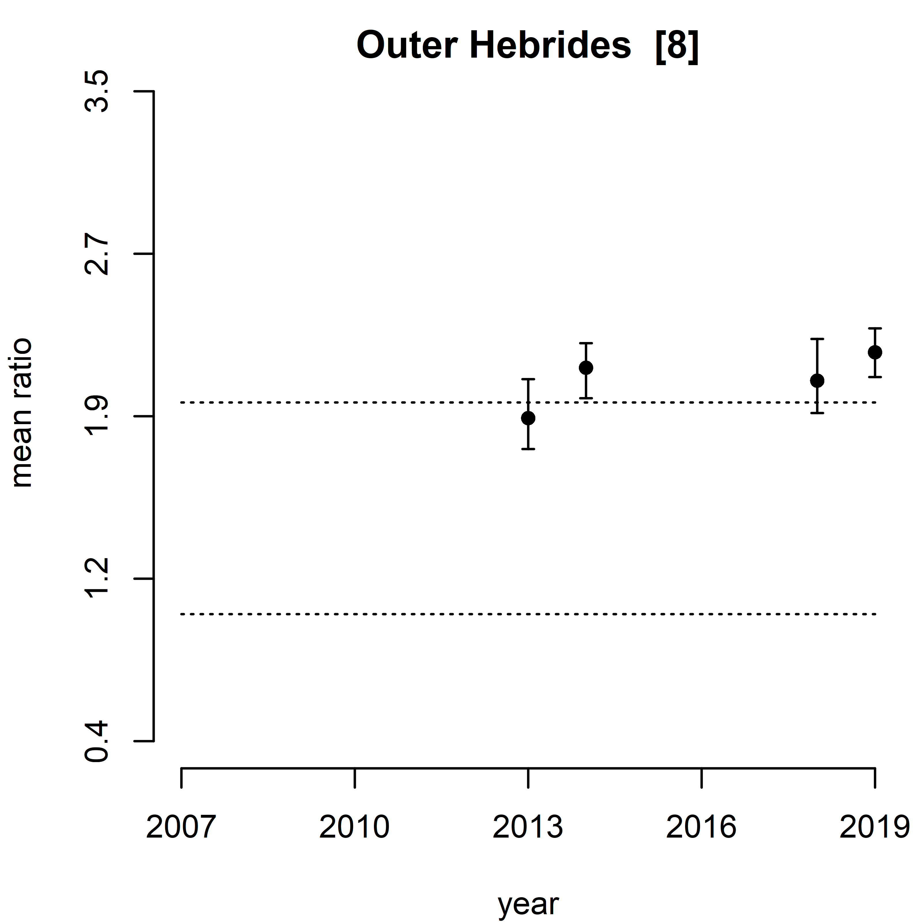
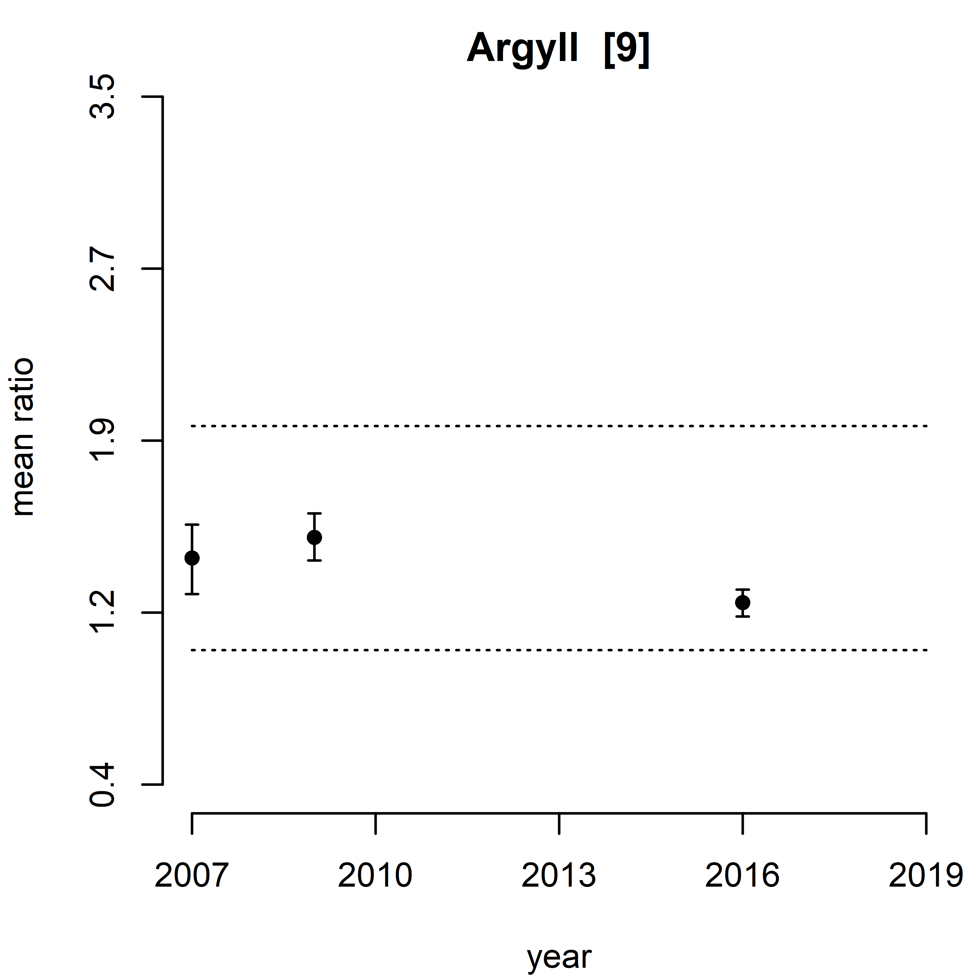
Figure d: Trend assessment of mean predicted salinity normalised TOxN for the 11 SMR regions between winters 2007 – 2019.

The offshore background concentration was exceeded in the Moray Firth, North East, Forth and Tay, North Coast and Shetland in 2010 & 2011 and in 2008 in the Forth and Tay (Figure d). This breach in offshore background concentrations may be as a consequence of the inflow of nutrient rich Atlantic waters to the system. Although the offshore background concentration was exceeded, the coastal background (12 µM) was not exceeded in any SMR.

No significant trend in normalised TOxN was observed in SMRs over the period of the assessment 2007 - 2019 (Figure d). The Orkney Islands were found to have increasing Total Nitrogen loads resulting in increasing nutrient inputs (see nutrient inputs assessment). This could be as a consequence of localised point sources such as aquaculture. The increased nitrogen load did not translate across to the wider marine region either because it was not readily available or there was dispersion/ dilution in the region. The Total Nitrogen load was also found to be significantly increasing in the Outer Hebrides (see nutrient inputs assessment). There were only 4 years of winter nutrient data available for the Outer Hebrides and therefore it should be noted a trend analysis was not possible (Figure d).

In UK waters there is no threshold for DIP, with DIP only being assessed as part of the TOxN to DIP (N/P) ratio. This is due to the nitrogen being the limiting nutrient in UK waters. Annual mean predicted DIP concentrations were low in all SMRs and all years, (Figure e). No statistically significant trend was observed in any SMR (Figure f).

Figure e: Mean predicted Dissolved Inorganic Phosphorous (DIP) in winter periods 20/07 – 2019 collected as part of the CSEMP annual monitoring cruise

Figure f. Trend assessment of mean predicted DIP for the 11 SMR regions between winters 2007 – 2019. There were no statistically significant trend in any of the regions.

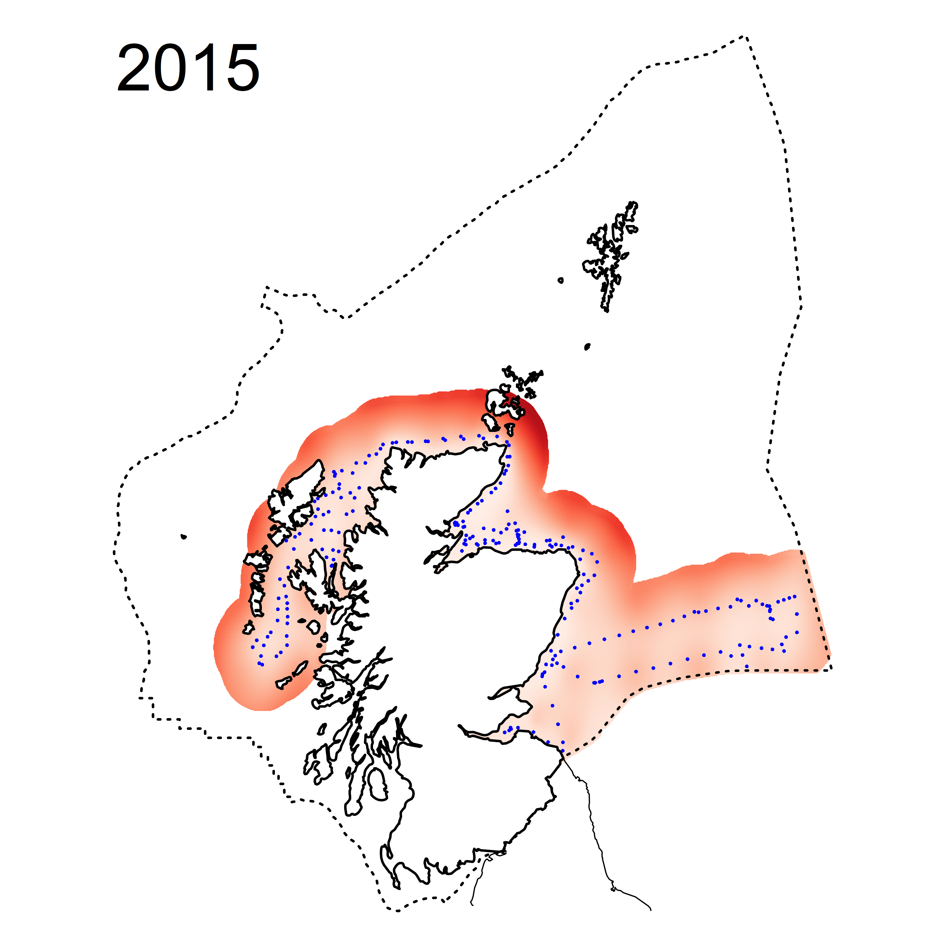
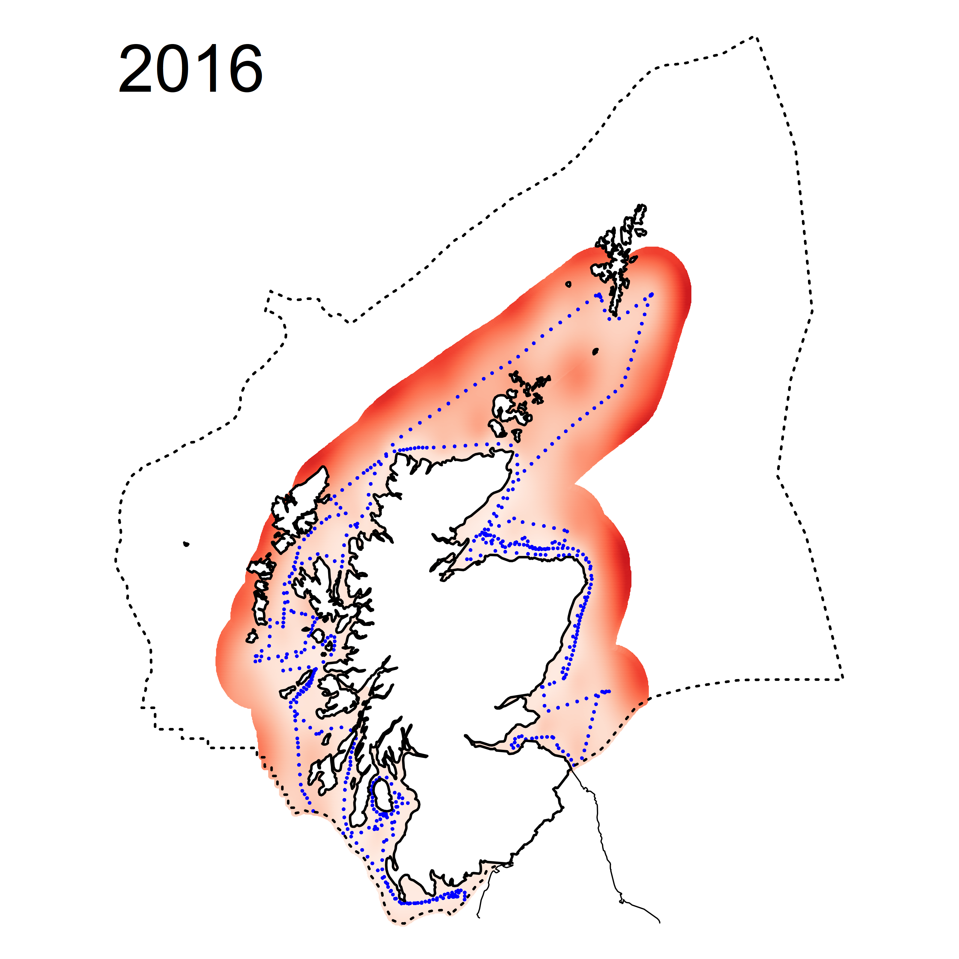
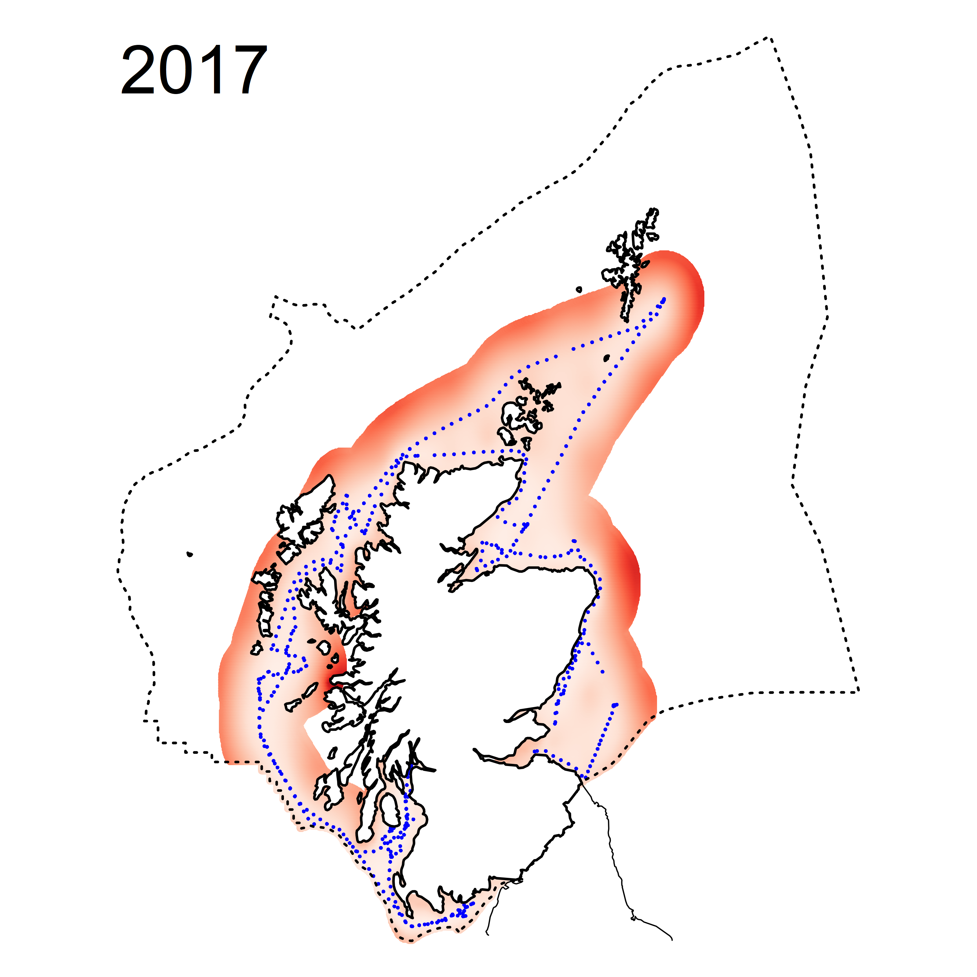
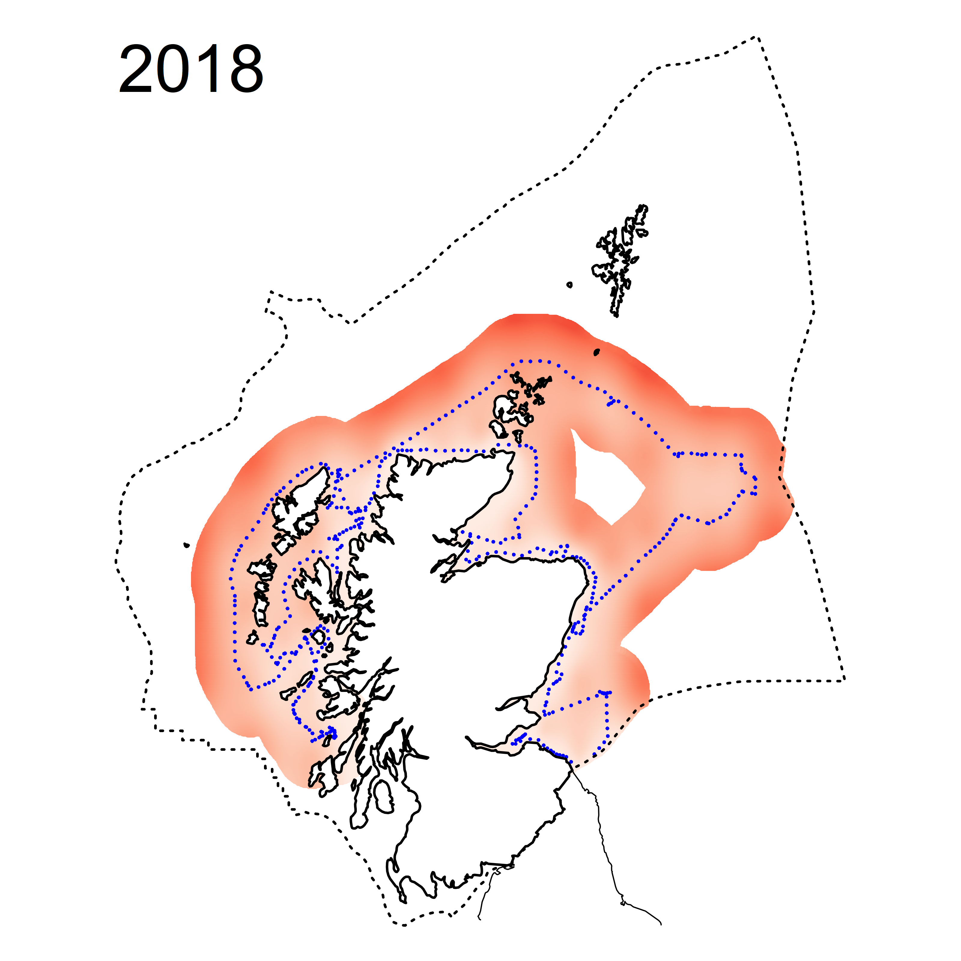
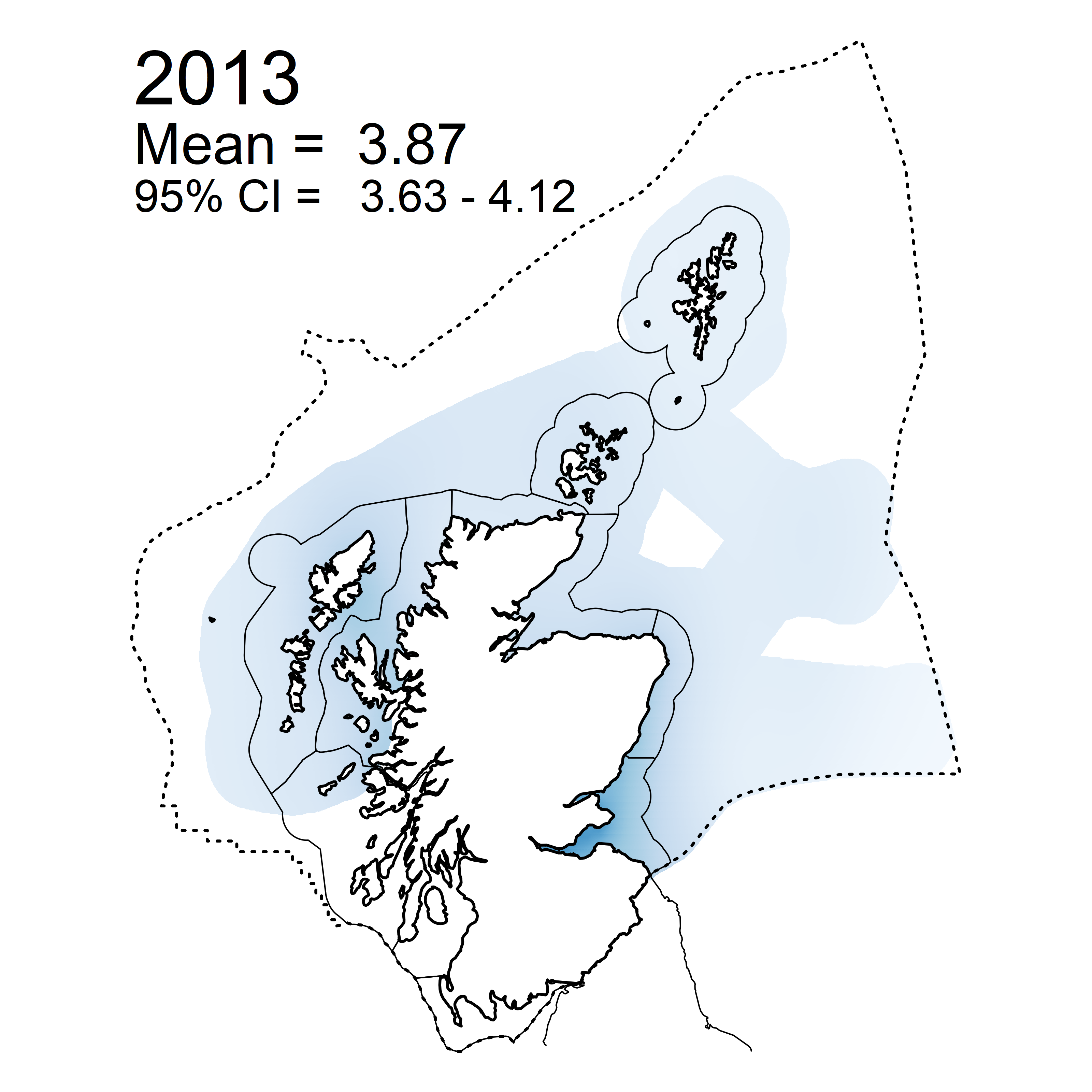
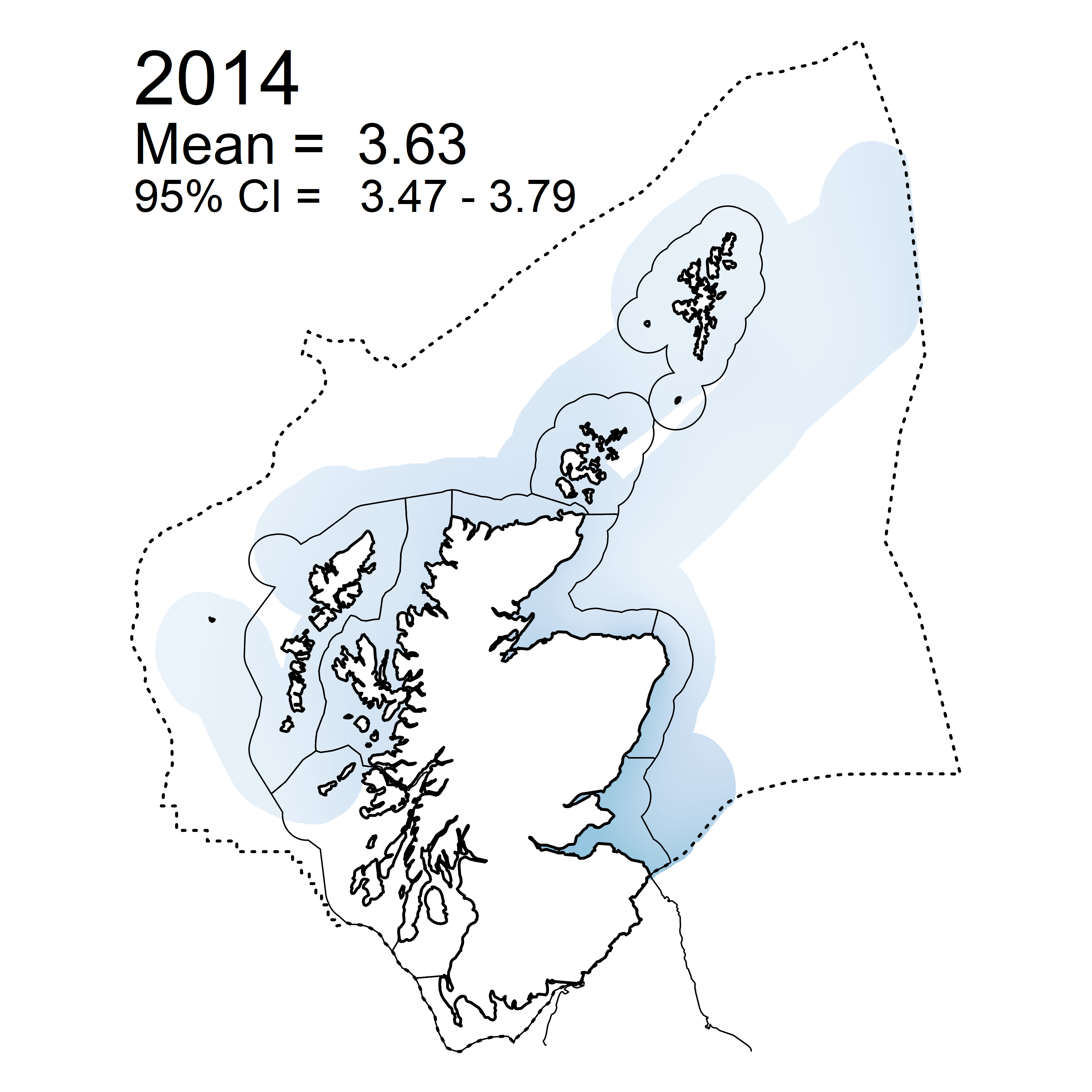
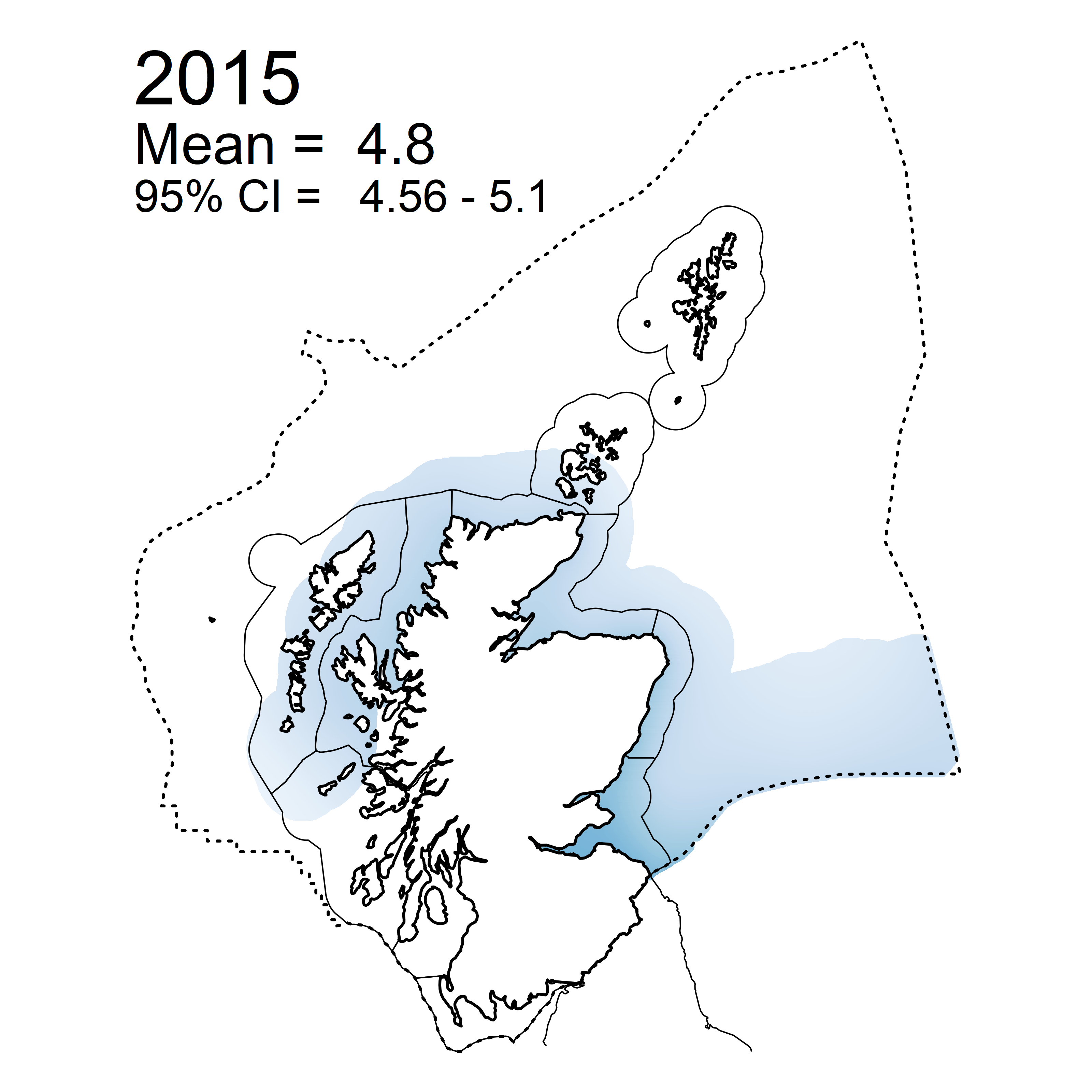
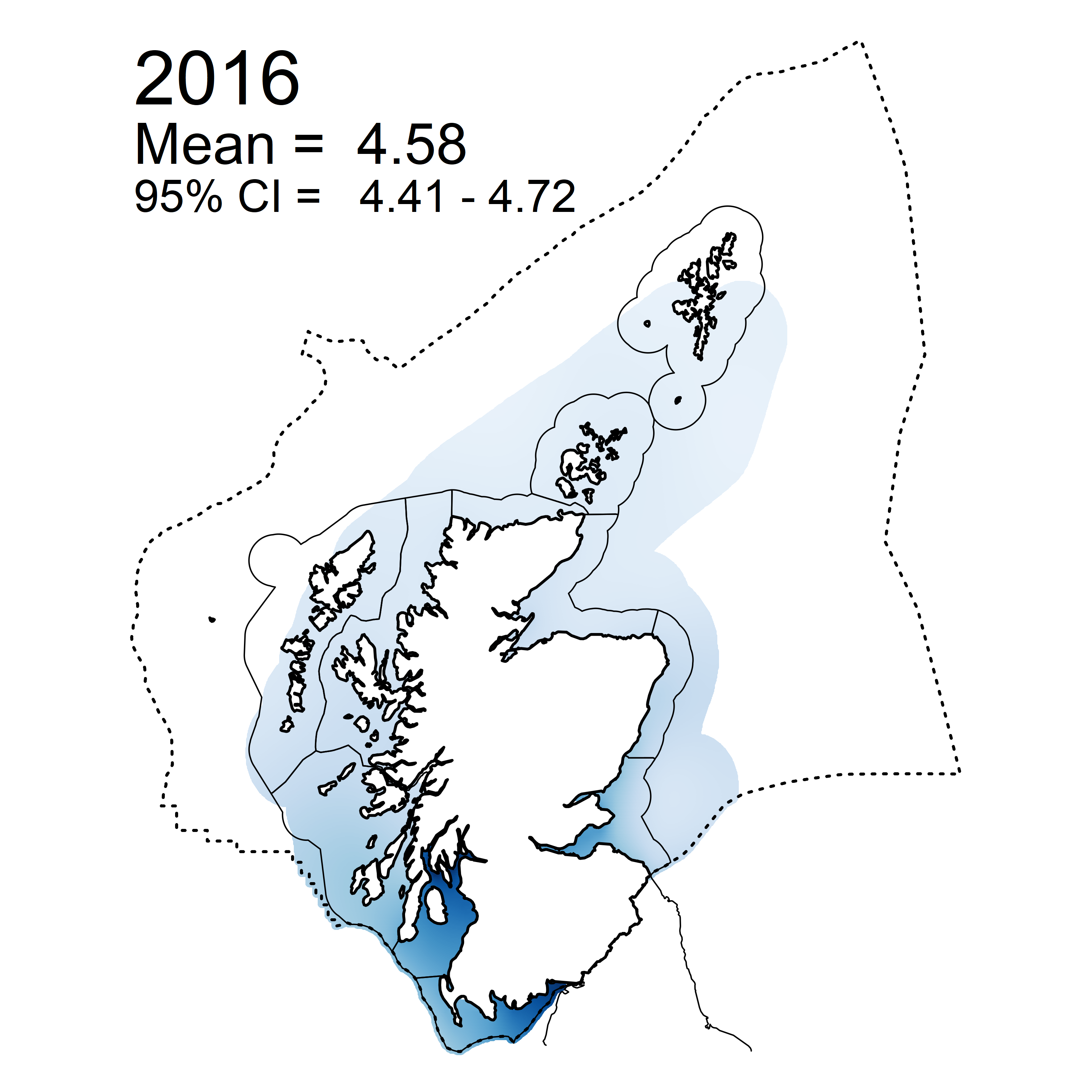
A significant trend in the predicted mean winter DSi was observed in 3 SMRs (Orkney Islands, North East and Forth and Tay), with decreases from 2015/16 onwards (Figure g).

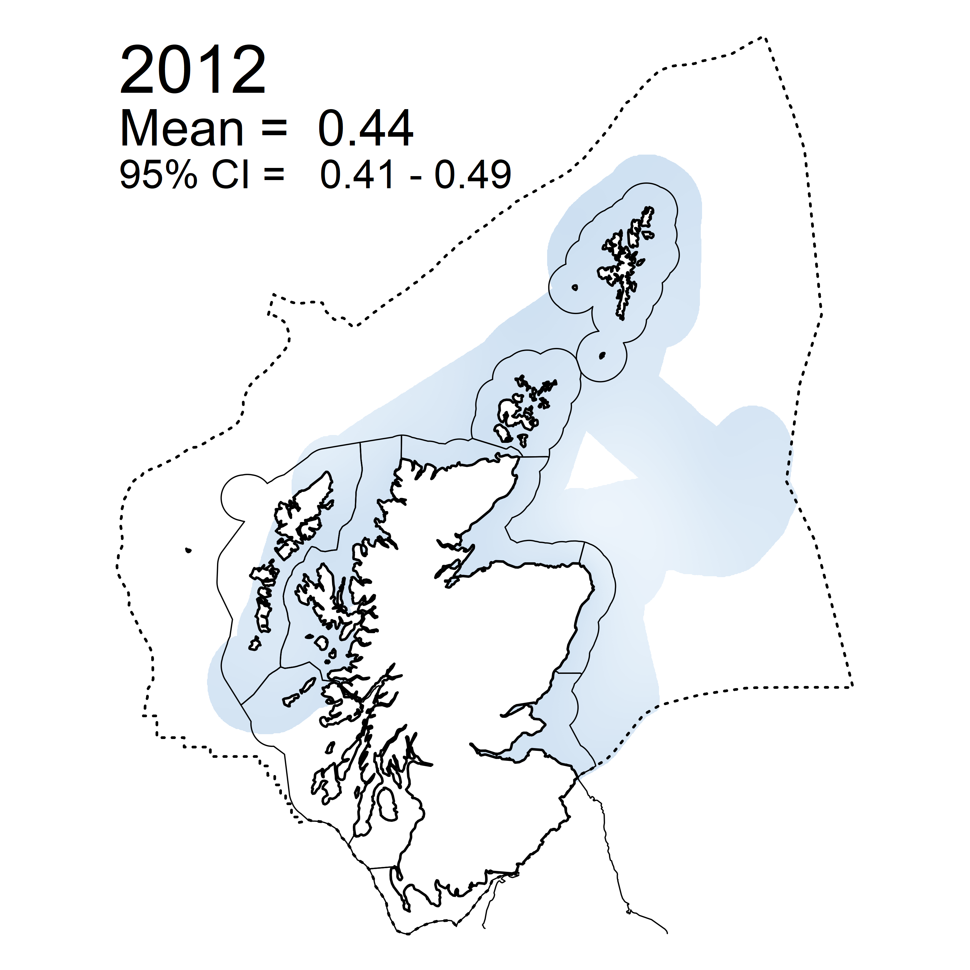
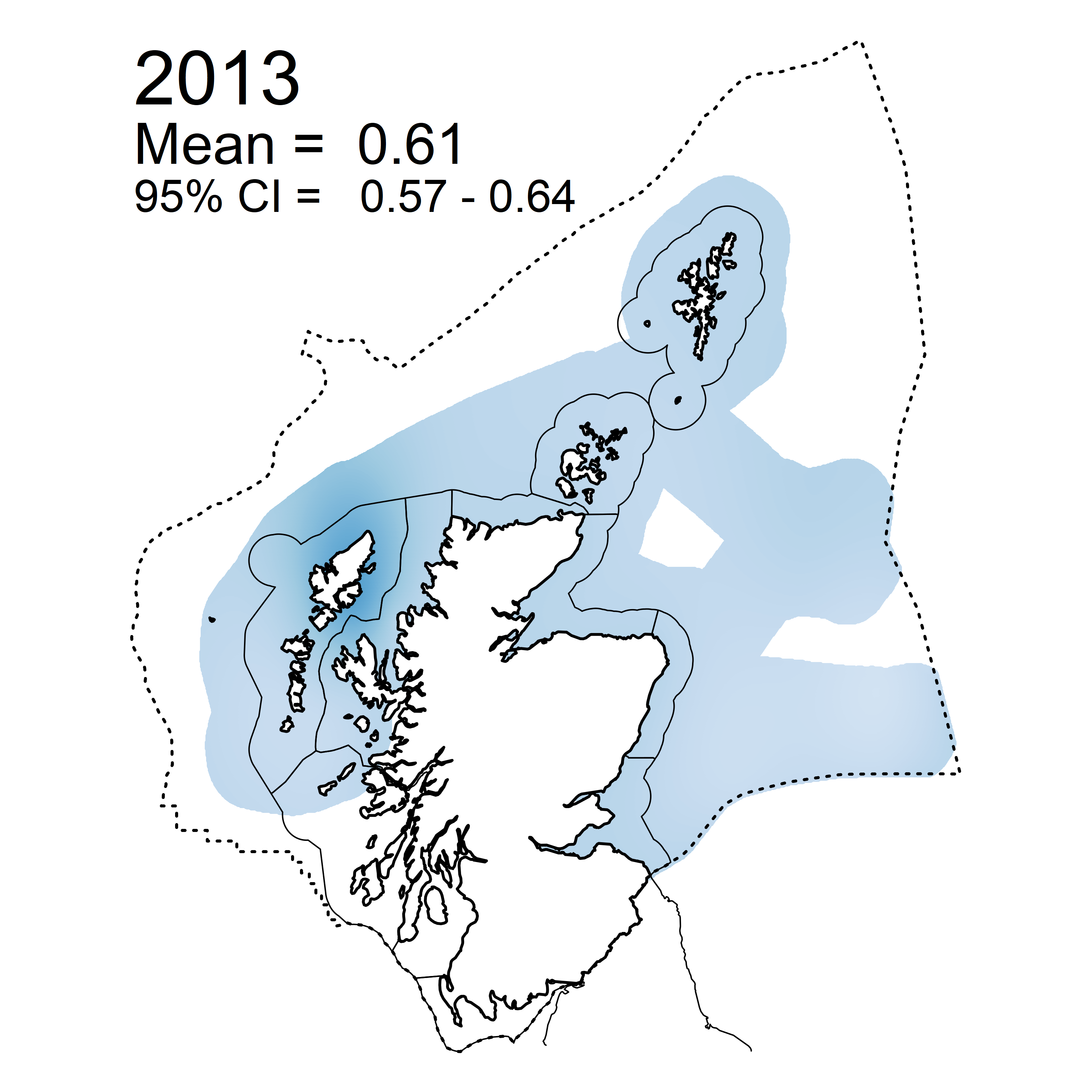
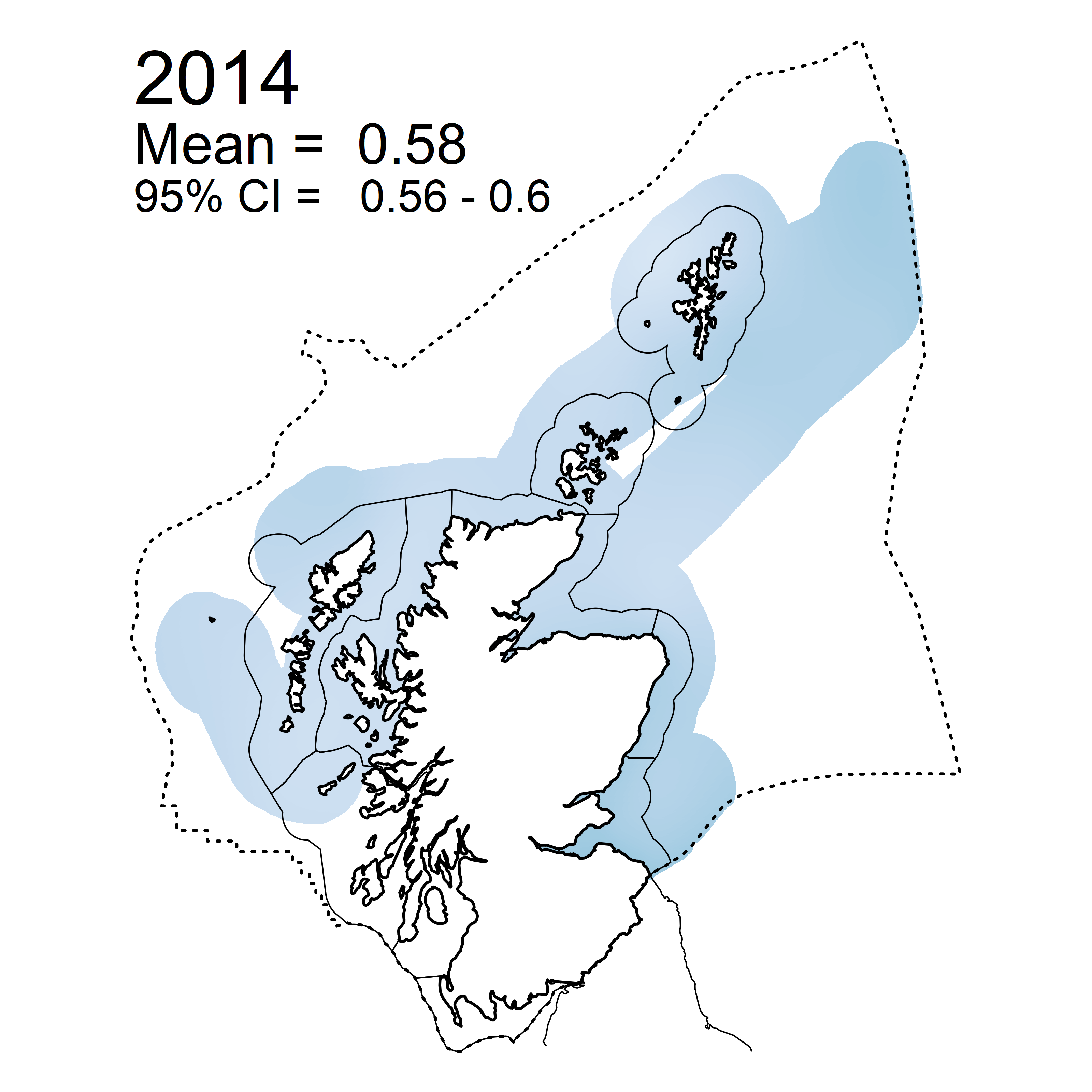
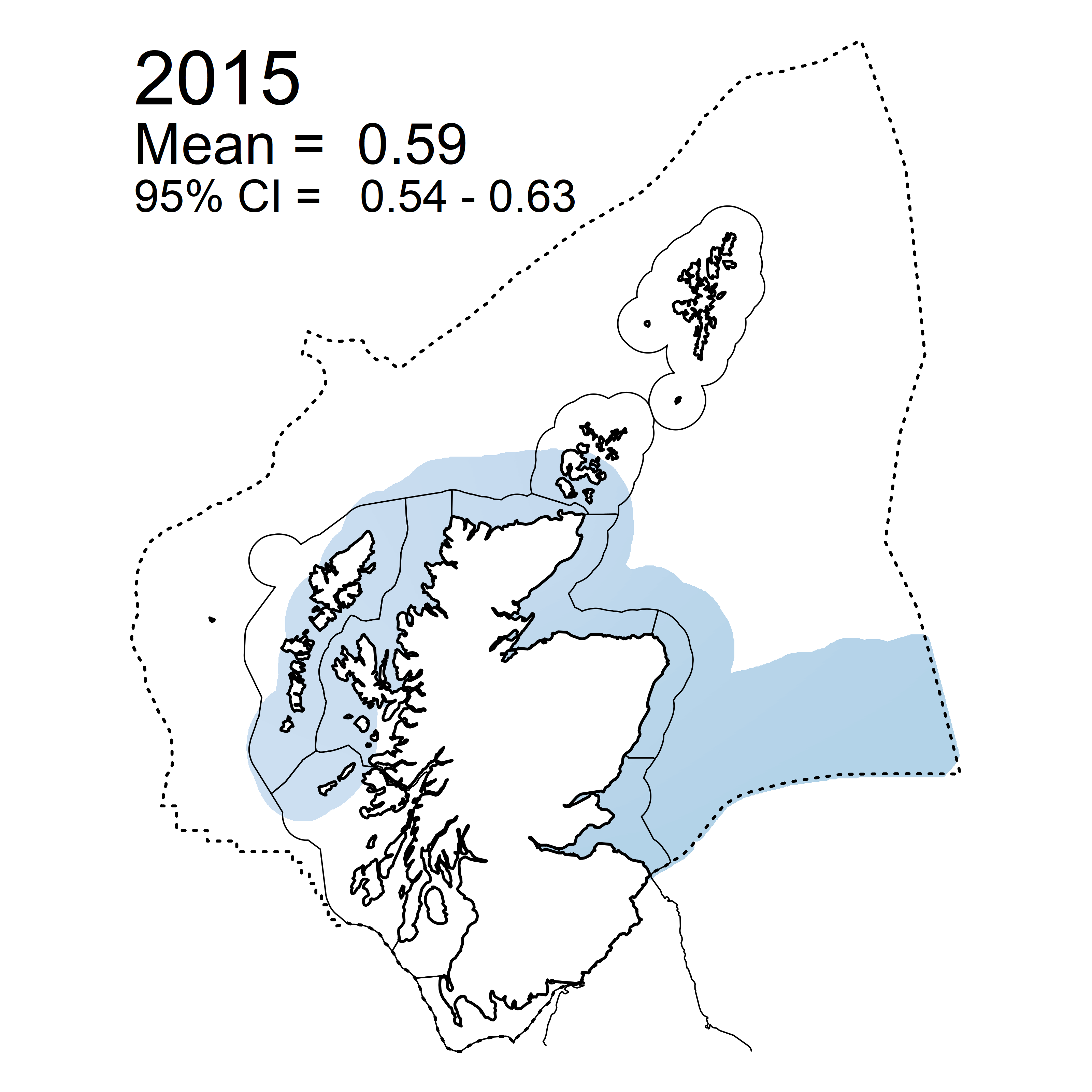
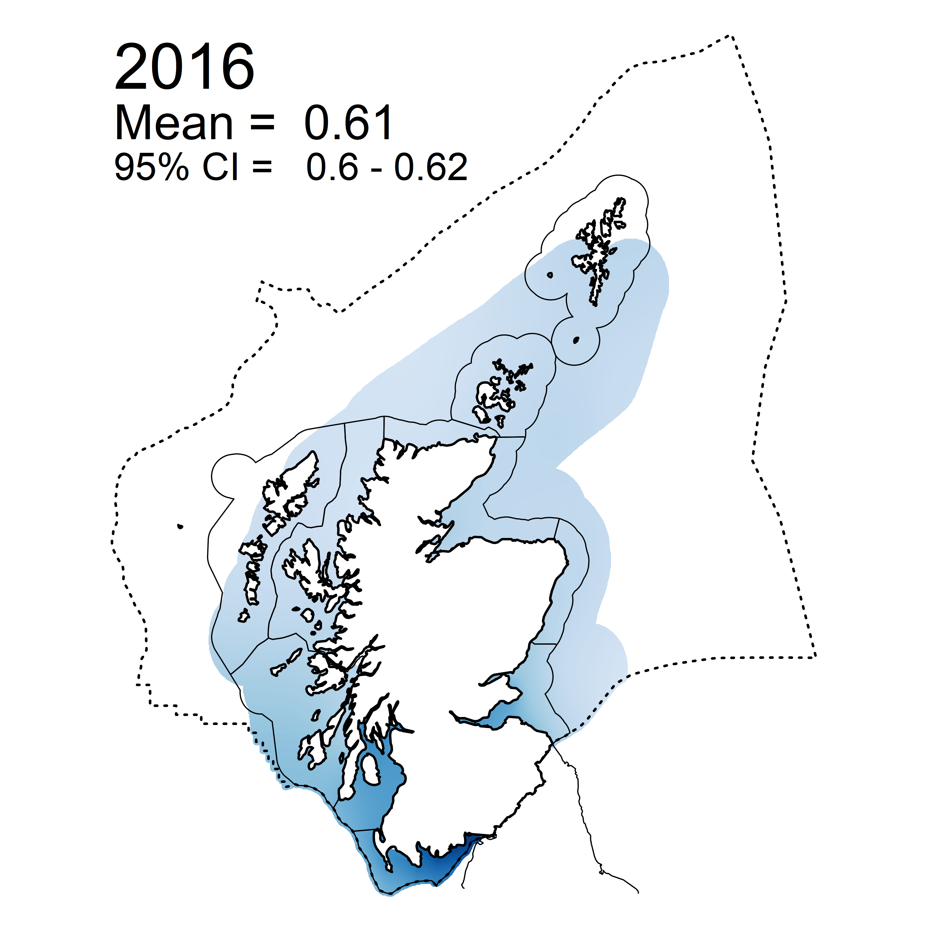
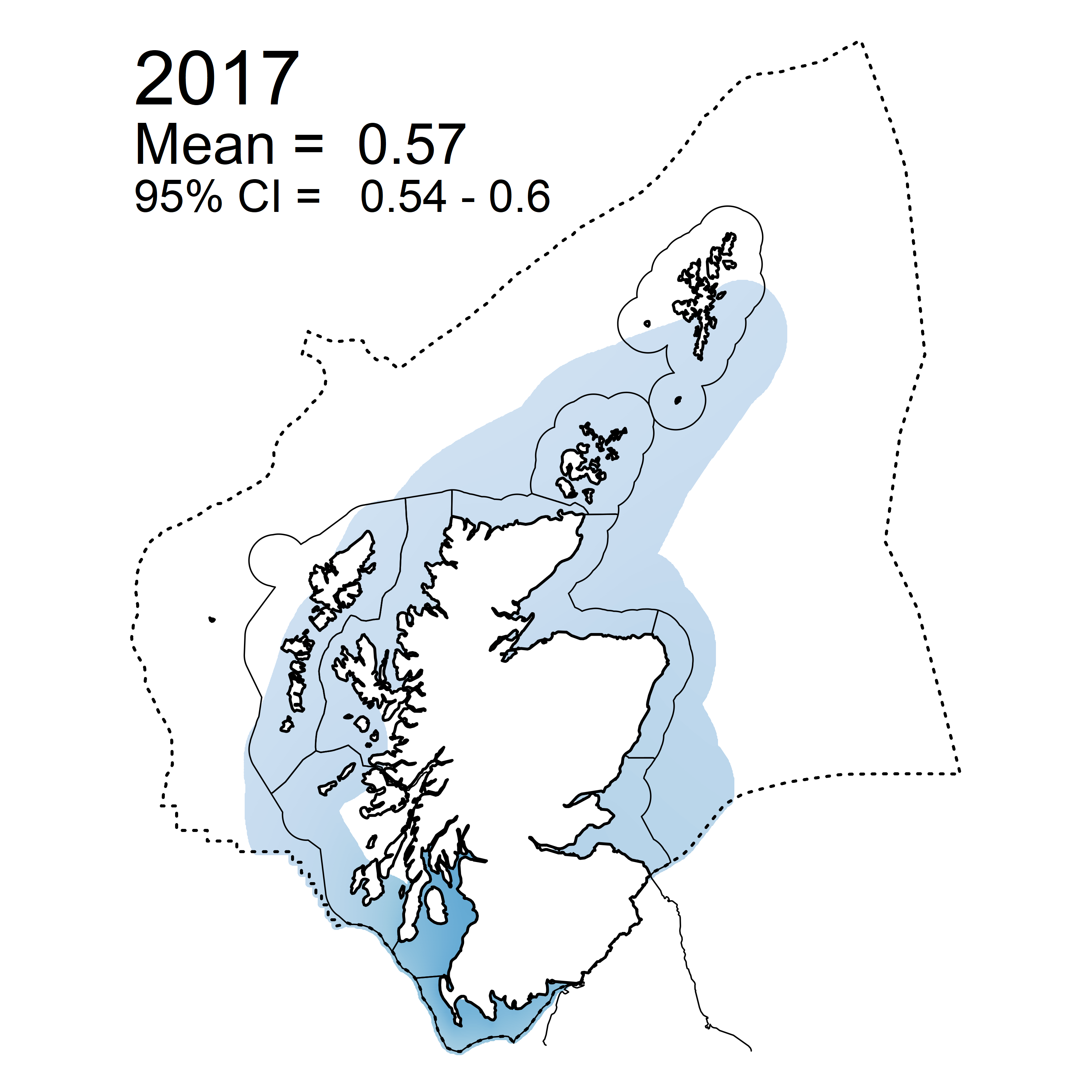
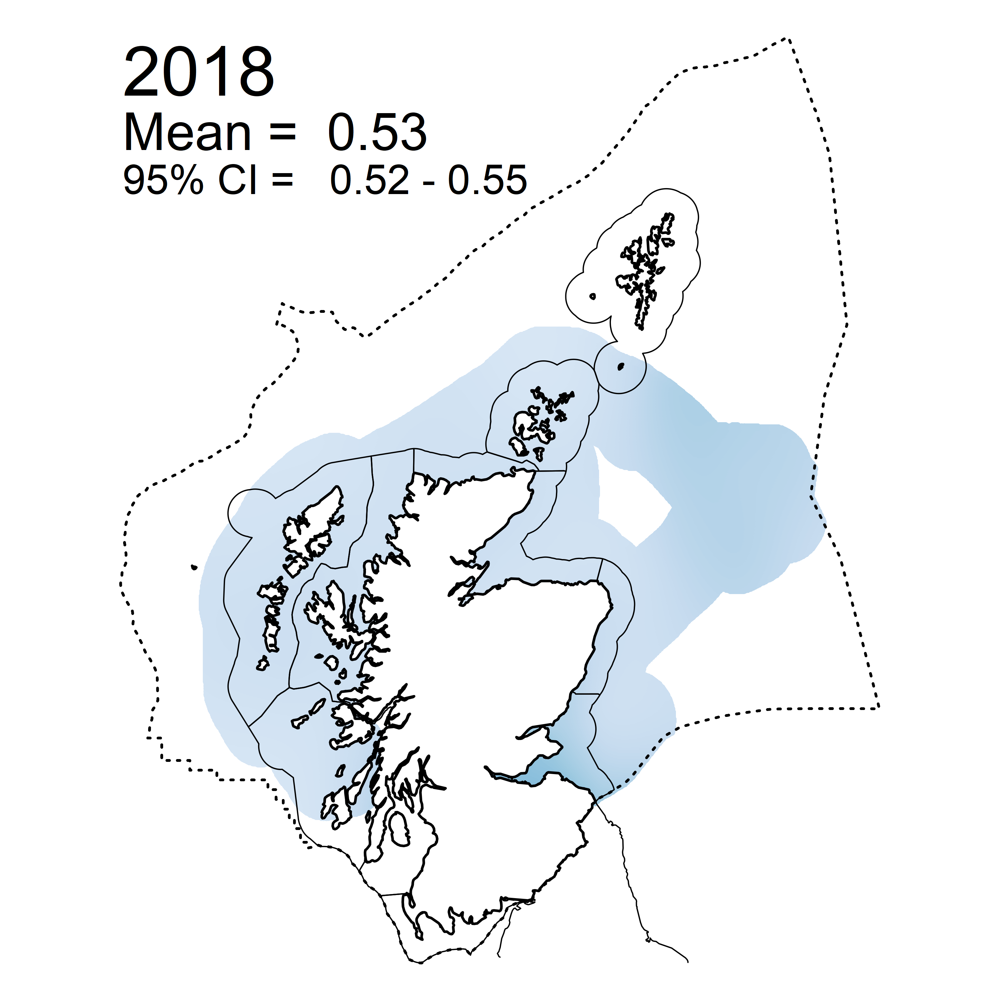
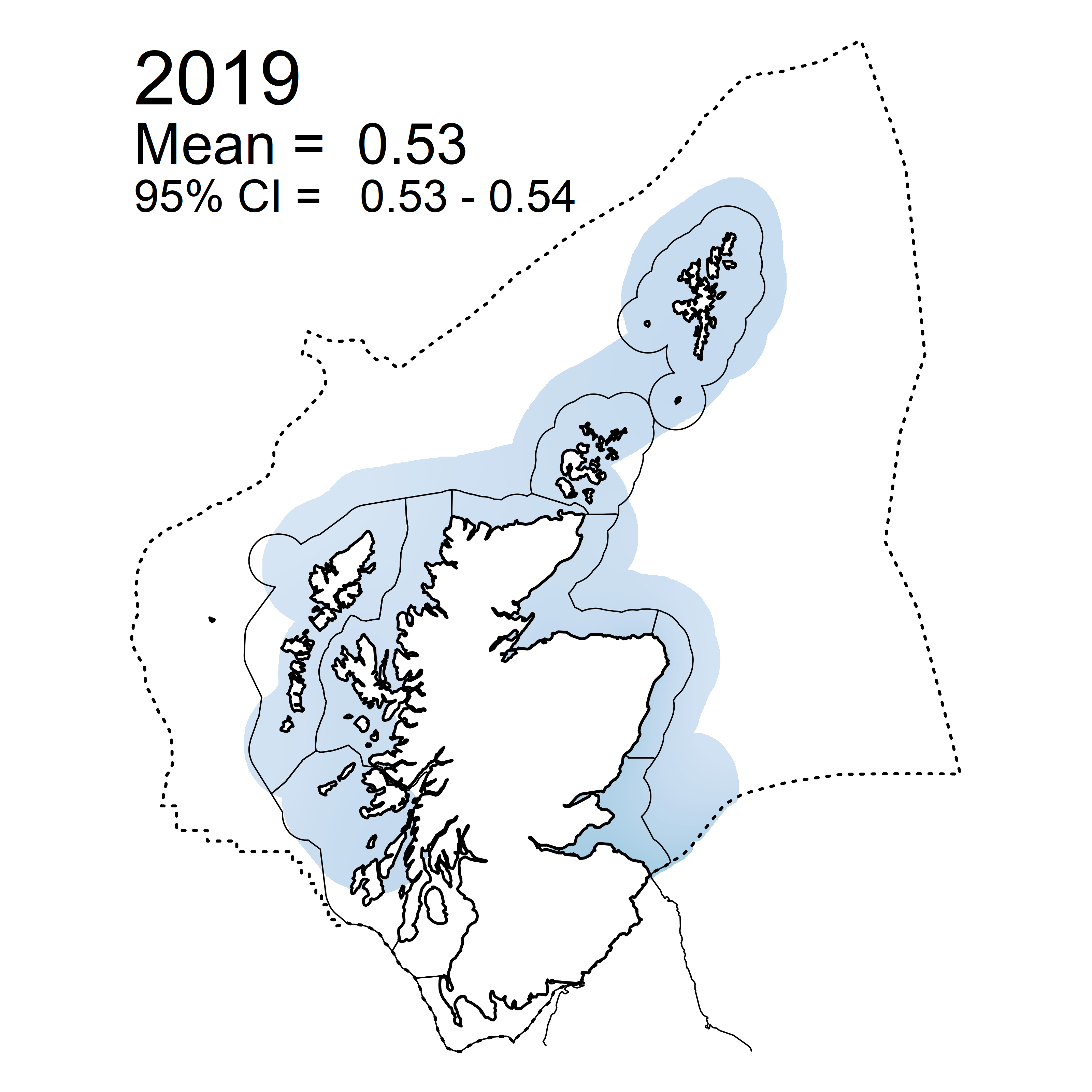
Figure g: Summary plot of modelled dissolved silicate (DSi) for winters 2007 – 2019. The Scottish Marine Regions (SMR) are identified as 1-11 corresponding to; SMR 1 Forth and Tay, SMR 2 North East, SMR 3 Moray Firth, SMR 4 Orkney Islands, SMR 5 Shetland Isles, SMR 6 North Coast, SMR 7 West Highlands, SMR 8 Outer Hebrides, SMR 9 Argyll, SMR 10 Clyde & SMR 11 Solway. Annual nutrient means with 95% confidence intervals (CI) for those SMR where predicted values covered at least 80% of the relevant area. Trends (continuous curvy line) with 95% CI (grey polygon) are shown only if the associated p-value is statistically significant.

There are no assessment criteria for DSi, with DSi only being assessed as part of the nitrogen to silicate (N/S) ratio. Predicted DSi concentrations were highest in the Forth and Tay, Clyde and Solway (Figure h). There is no causal link to nutrient inputs and this may be linked to local geology. A statistically significant trend was observed in three SMRs, namely Orkney Islands, North East and Forth and Tay (Figure i). In the Forth and Tay region predicted mean annual concentrations appear to increase to a maxima around the winter 2012, while in the North East and Orkney Islands the maxima is around 2015 and 2011 respectively (Figure i). In all three regions this maxima was followed by concentrations decreasing to those observed at the start of the time period (Figure i).

Figure h: Mean predicted Dissolved Inorganic Silicate (DSi) in winter periods 2007 – 2019 collected as part of the CSEMP annual monitoring cruise.

Figure i: Trend assessment of mean predicted DSi for the 11 SMR regions between winters 2007 – 2019. There were no statistically significant trend in any of the regions.

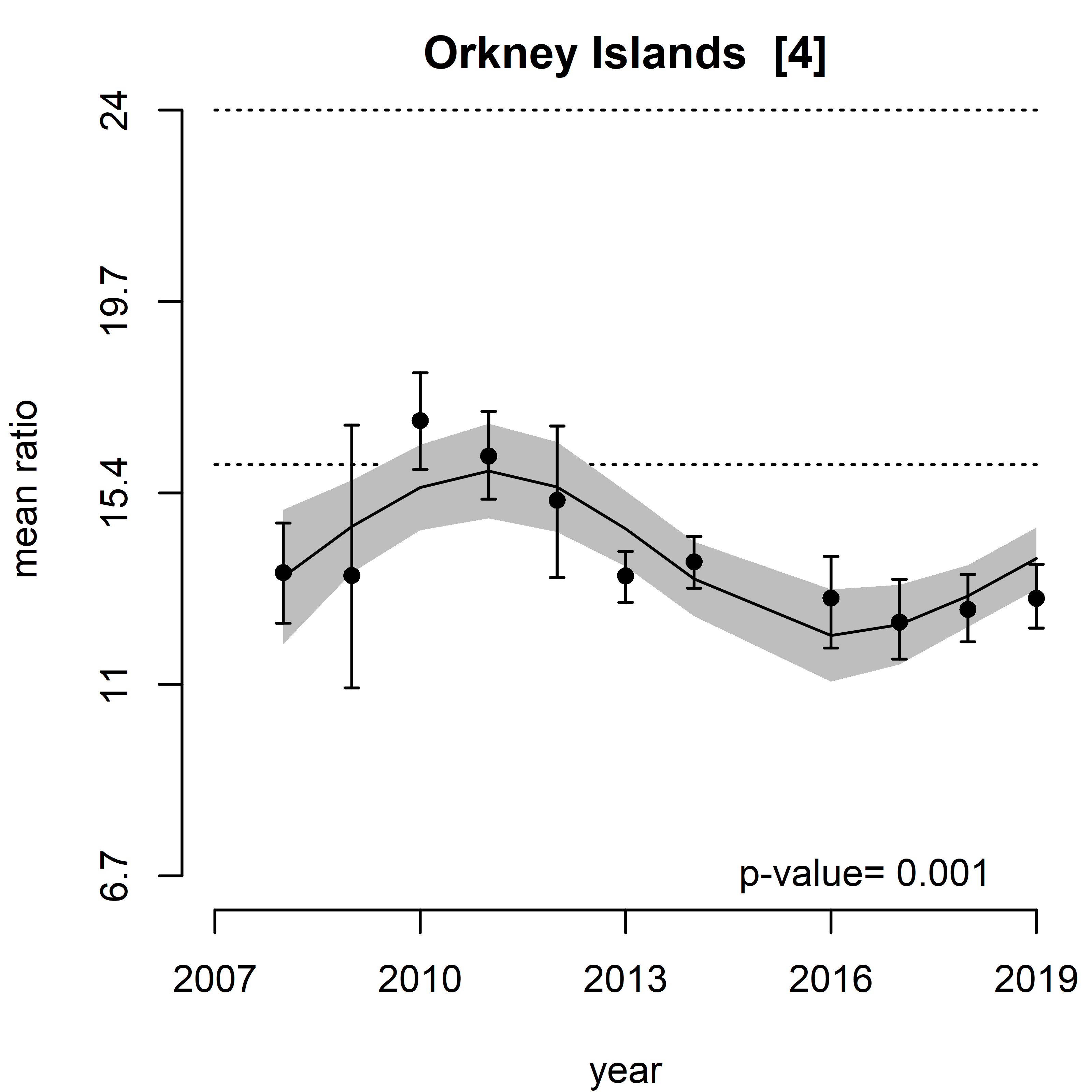
The mean predicted N/P ratio was below the elevated assessment value of 24 in all SMRs, with significant trends being observed in the Orkney Islands. In this region the N/P ratio increased to maximise between winter 2010 – 2013 before decreasing to a steady state thereafter (Figure j).

Figure j: Summary plot of predicted N/P ratios for winters 2007-2019 along with the predicted trend assessment for the time series (2007-2019). The Scottish Marine Regions (SMR) are identified as 1-11 corresponding to; SMR 1 Forth and Tay, SMR 2 North East, SMR 3 Moray Firth, SMR 4 Orkney Islands, SMR 5 Shetland Isles, SMR 6 North Coast, SMR 7 West Highlands, SMR 8 Outer Hebrides, SMR 9 Argyll, SMR 10 Clyde & SMR 11 Solway. Annual nutrient means with 95% confidence intervals (CI) for those SMR where predicted values covered at least 80% of the relevant area. Trends (continuous curvy line) with 95% CI (grey polygon) are shown only if the associated p-value is statistically significant. The hashed lines, in the trend assessment, correspond to offshore background (16) and assessment level (24) ratios for winter offshore N/P.

Across the assessment area, predicted mean annual N/P ratio were found to be below the elevated ECoQO for the N/P ratio of 24 (Figure k). The mean N/P ratio exceeded the background ECoQOs (16) in 2010, 2011 & 2013 (Figure k). The highest predicted ratio was for the north of the Outer Hebrides SMR in 2007 (Figure k). However, 2007 is also the year where there is the least confidence in the predicted N/P ratio (Figure l) due to reduced sampling as a result of bad weather and data should be treated with caution. A statistically significant trend in the N/P ratio was observed in one SMR (Orkney Islands; Figure m). In this region the N/P ratio increased to maximise between winter 2010 - 2013 before decreasing to a steady state thereafter (Figure m). There is no apparent causal linkage to the nutrient inputs or predicted concentrations and therefore must either be due to an unidentified biological event or analytical or modelling effects. During the period 2010 – 2013, mean annual N/P ratio was highest ( > background) in the Shetland Islands, but below the assessment level of 24 (Figure m).

Figure k: Mean predicted N/P ratio in winter periods 2007 – 2019 collected as part of the CSEMP annual monitoring cruise.

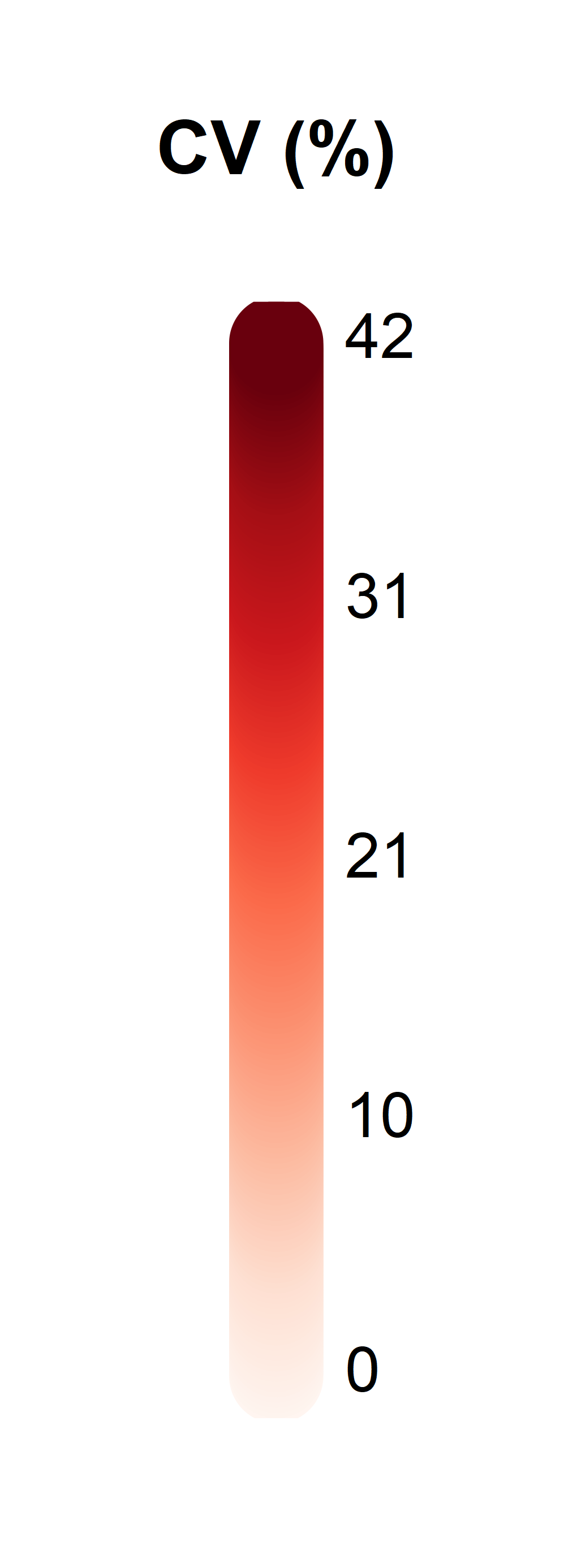Figure l: Coefficient of variation (CV%) of the modelled data set for N/P ratio. With least accuracy found on the outer boundaries furthest from sampling position.

Figure m: Trend assessment of mean predicted N/P ratio for the 11 SMR regions between winters 2007 – 2019. Annual nutrient means with 95% confidence intervals (CI) for those SMR where predicted values covered at least 80% of the relevant area. Trends (continuous curvy line) with 95% CI (grey polygon) are shown only if the associated p-value is statistically significant. The hashed lines, in the trend assessment, correspond to background (16) and assessment level (24) ratios for winter offshore N/P.

As described previously there is no assessment criteria for DSi and it is only being assessed as part of the nitrogen to silicate (N/S) ratio. The OSPAR N/S background and elevated ratios are 1 and 2 respectively. The N/S ratio exceeded the background assessment in all SMRs and years (Figure n). This has previously been attributed to low silicate Atlantic waters entering the shelf seas (Smith et al., 2014). The authors concluded in their assessment, that highest N/S ratios were found in regions influenced by Atlantic water, with lower ratios along the coast and near river mouths. In this study the highest N/S ratio was found in the Shetland Islands which is strongly influenced by Atlantic water. Smith et al.,(2014) suggested the OSPAR background and elevated N/S ratios were not appropriate for Scottish Shelf Seas and proposed an alternative derived from data from the Minches and Malin Sea of 1.7 (background) and 3.4 (elevated). Assessing this dataset against the proposed Scottish N/S ratio, a number of regions would still have exceeded background levels, particularly those strongly influenced by Atlantic waters, namely: the Orkney Islands, Shetland Islands and the Outer Hebrides SMRs (Figure n) and further investigation into the N/S ratios is merited.

Figure n: Trend assessment of mean predicted N/S ratio for the 11 SMR regions between winters 2007 – 2019. Annual nutrient means with 95% confidence intervals (CI) for those SMR where predicted values covered at least 80% of the relevant area. The hashed lines, in the trend assessment, correspond to offshore background (1) and assessment level (2) ratios for winter offshore N/S.

Reported data in this assessment are comparable with the assessment undertaken for the Third Integrated Report on the Eutrophication Status of the OSPAR Maritime area (OSPAR, 2017), where DIN did not exceed the assessment level in the Greater North Sea.

Results from WFD classification have highlight elevated DIN concentrations in two estuarine waterbodies: The River Ythan estuary (North East SMR) and the Inner Clyde Estuary (Clyde SMR). However, DIN concentrations were not found to be elevated in either these SMRs indicating this was a localised impact.

The data are also comparable for winter nutrients collected as part of the Scottish Coastal Observatory Monitoring Program (Bresnan et al., 2016).

Although a regional assessment of status was not undertaken for the Scottish Marine Atlas in 2011, winter nutrient data were presented as part of the eutrophication assessment. Only winter DIN was considered for the assessment, and concentrations were below the elevated threshold in offshore and most coastal waters. Assessment was based on discrete samples only with no modelling undertaken across Scottish Sea areas.

Conclusion

The eleven Scottish Marine Regions have been assessed for winter nutrient concentrations. Discrete water samples were collected in January of each year, between 2007-2019, and the data used to model nutrient concentrations and assess trends. There were no statistically significant increase in the winter nutrient concentrations during the period 2007 to 2019 in any of the regions and concentrations are consistently below the OSPAR EcoQO.

The assessment of nutrient inputs found nutrients were increasing in the Outer Hebrides and Orkney Islands, but this did not translate across to increased winter nutrients in these regions.

Similar to the study of Smith et al. (2014), the OSPAR nitrogen to silicate (N/S) background and elevated ratios of 1 and 2 respectively, were found to be inappropriate to the Scottish Shelf seas, where winter silicate concentrations are low due to the influence of Atlantic waters, resulting in ratios above 2. The highest ratios of N/S in our assessment were in regions most strongly influenced by Atlantic waters such as the Shetland SMR.

Knowledge gaps

Winter nutrient monitoring on the annual CSEMP cruise is well established but does not include collection from all SMRs. The nutrient inputs assessment found increasing nutrients in both the Outer Hebrides and Orkney Island SMRs. Winter nutrient concentrations, in the years assessed, were below elevated ECoQO thresholds in both these SMRs, although it should be noted data coverage for the Outer Hebrides SMR is limited.

The Orkney Island region was found to have a statistically significant increased N/P ratio which maximised between winter 2010- 2013 before decreasing. This phenomenon is not understood.

There are limited winter nutrient monitoring data available for the Clyde, Solway, Outer Hebrides and Shetland Islands (in more recent years). This is because the design of the sampling is around the contaminants and effects monitoring in sediment and fish with opportunistic collection of water for nutrients.

Two SMRs were found, in the nutrient inputs assessment, to have increasing nutrient loads. However, this did not translate across to increased winter nutrients in these regions in this assessment, but may affect the regions in the future. There is limited winter nutrient data available, in particular for the Outer Hebrides, and therefore increased winter nutrient monitoring in the Orkney Islands and Outer Hebrides may be necessary.

Consideration should be given as to whether it is necessary to continue annual monitoring in regions where there is a large dataset and alter the sampling programme to address regions with limited data.

The N/P ratio was increased in the Orkney Islands to maximise between winter 2010- 2013 before decreasing to a steady state thereafter. There was no causal linkage to the nutrient inputs or predicted concentrations and therefore the increase must either have been due to an unidentified biological event, or analytical or modelling effects. This unknown event is a gap in our current understanding.

The OSPAR N/S background and elevated ratios of 1 and 2 respectively, are inappropriate to the Scottish Shelf seas, which are strongly influenced by Atlantic waters. Smith et al. (2014) previously proposed an alternative derived from data from the Minches and Malin Sea of 1.7 (background) and 3.4 (elevated). These ratios may still be too low for areas such as the Shetland Islands and further investigation is merited.

Status and trend assessment

The status and trend assessment is for eutrophication and includes, nutrient inputs, winter nutrient concentrations, chlorophyll concentrations and dissolved oxygen concentrations.

Region assessed	Status with confidence	Trend with confidence	Comments
Argyll			Status and trends have been given a confidence of 2 stars because there is limited dissolved oxygen data available in the region and this has been acknowledged as a knowledge gap in the current assessment of overall Eutrophication status
Clyde			The status green box with blue circle is due to a localised issue within the inner Clyde estuary where the dissolved oxygen is failing. Status and trends have been given a confidence of 2 stars because there is limited dissolved oxygen data available in the region and this has been acknowledged as a knowledge gap in the current assessment of overall Eutrophication status.
Forth and Tay			Status and trends have been given a confidence of 2 stars because there is limited dissolved oxygen data available in the region and this has been acknowledged as a knowledge gap in the current assessment of overall Eutrophication status. There is a localised issue with the trend assessment due to increasing chlorophyll concentrations, but trend not reflected in other eutrophication parameters.
Moray Firth			Status and trends have been given a confidence of 2 stars because there is limited dissolved oxygen data available in the region and this has been acknowledged as a knowledge gap in the current assessment of overall Eutrophication status.
North Coast			Status and trends have been given a confidence of 2 stars because there is limited dissolved oxygen data available in the region and this has been acknowledged as a knowledge gap in the current assessment of overall Eutrophication status.
North East			The status green box with blue circle is due to a localised issue within the Ythan Estuary which is categorised as being eutrophic. The rest of the SMR is not impacted and not considered to be Eutrophic. Status and trends have been given a confidence of 2 stars because there is limited dissolved oxygen data available in the region and this has been acknowledged as a knowledge gap in the current assessment of overall Eutrophication status.
Orkney Islands			Status and trends have been given a confidence of 2 stars because there is limited dissolved oxygen data available in the region and this has been acknowledged as a knowledge gap in the current assessment of overall Eutrophication status. There is a localised issue of increasing nutrient inputs in the region associated with increasing aquaculture. This increasing input is not impacting nutrients across the SMR with no statistically significant trend in winter DIN observed.
Outer Hebrides			There is a localised issue of increasing nutrient inputs in the region associated with increasing aquaculture. This increasing input is not impacting nutrients across the SMR with no statistically significant trend in winter DIN observed. Status and trends have been given a confidence of 2 stars because there is limited dissolved oxygen data available in the region and this has been acknowledged as a knowledge gap in the current assessment of overall Eutrophication status.
Shetland Isles			Status and trends have been given a confidence of 2 stars because there is limited dissolved oxygen data available in the region and this has been acknowledged as a knowledge gap in the current assessment of overall Eutrophication status.
Solway			Status and trends have been given a confidence of 2 stars because there is limited dissolved oxygen data available in the region and this has been acknowledged as a knowledge gap in the current assessment of overall Eutrophication status.
Western Islands			Status and trends have been given a confidence of 2 stars because there is limited dissolved oxygen data available in the region and this has been acknowledged as a knowledge gap in the current assessment of overall Eutrophication status.

This Legend block contains the key for the status and trend assessment, the confidence assessment and the assessment regions (SMRs and OMRs or other regions used). More information on the various regions used in SMA2020 is available on the Assessment processes and methods page.

Status and trend assessment

Status assessment (for Clean and safe, Healthy and biologically diverse assessments)		Trend assessment (for Clean and safe, Healthy and biologically diverse and Productive assessments)
	Many concerns		No / little change
	Some concerns		Increasing
	Few or no concerns		Decreasing
	Few or no concerns, but some local concerns		No trend discernible
	Few or no concerns, but many local concerns		All trends
	Some concerns, but many local concerns
	Lack of evidence / robust assessment criteria
	Lack of regional evidence / robust assessment criteria, but no or few concerns for some local areas
	Lack of regional evidence / robust assessment criteria, but some concerns for some local areas
	Lack of regional evidence / robust assessment criteria, but many concerns for some local areas

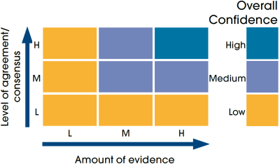
Confidence assessment

Symbol	Confidence rating
	Low
	Medium
	High

Assessment regions

The Scottish Marine Regions (SMRs; S1 – S11) and the Scottish Offshore Marine Regions (OMRs, O1 – O10)

Key: S1, Forth and Tay; S2, North East; S3, Moray Firth; S4 Orkney Islands, S5, Shetland Isles; S6, North Coast; S7, West Highlands; S8, Outer Hebrides; S9, Argyll; S10, Clyde; S11, Solway; O1, Long Forties, O2, Fladen and Moray Firth Offshore; O3, East Shetland Shelf; O4, North and West Shetland Shelf; O5, Faroe-Shetland Channel; O6, North Scotland Shelf; O7, Hebrides Shelf; O8, Bailey; O9, Rockall; O10, Hatton.

Biogeographic, Charting Progress 2 (CP2) Regions. These have been used as the assessment areas for hazardous substances.

Scottish Sea Areas as used in Scotland's Marine Atlas 2011. These are sub divisions of the biogeographic, or Charting Progress 2 (CP2), Regions.

Sections

Key message

Background

Background (Extended)

Assessment methods

Description of data

Winter Nutrient Concentration Assessment and Geographical Scale

Data Preparation

Results

Results (Extended)

Conclusion

Conclusion (Extended)

Knowledge gaps

Knowledge gaps (Extended)

Status and trend assessment

Legend

Status and trend assessment

Confidence assessment

Assessment regions

Links and resources